
Assignment #3 STA355H1S

Assignment代写 Instructions: Solutions to problems 1 and 2 are to be submitted on Quercus (PDF files only) – the deadline is 11:59pm
due Friday March 22, 2019
Instructions: Solutions to problems 1 and 2 are to be submitted on Quercus (PDF files only) – the deadline is 11:59pm on March 22. You are strongly encouraged to do problems 3 through 6 but these are not to be submitted for grading.
Problems to hand in:
1.Supposethat D1, · · , Dn are random directions Assignment代写
– we can think of these random variables as coming from a distribution on the unit circle {(x, y) : x2 + y2 = 1} and represent each observation as an angle so that D1, · · · , Dn come from a distribution on [0, 2π). (Directional or circular data, which indicate direction or cyclical time, can be of great interest to biologists, geographers, geologists, and social scientists. The defining characteristic of such data is that the beginning and end of their scales meet so, for example, a direction of 5 degrees is closer to 355 degrees than it is to 40 degrees.)Assignment代写
A simple family of distributions for these circular data is the von Mises distribution whose density on [0, 2π) is
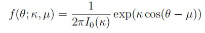
where 0 ≤ µ < 2π, κ ≥ 0, and I0(κ) is a 0-th order modified Bessel function of the first kind:
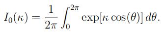
(In R, I0(κ) can be evaluated by besselI(kappa,0).) Note that when κ = 0, we have a uniform distribution on [0, 2π) (independent of µ).
(a)Show that the MLE of µsatisfies Assignment代写
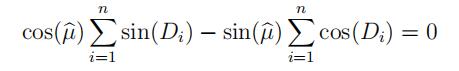
and give an explicit formula for µ in terms of Σ sin(Di) and Σ cos(Di). (Hint: Use the
formula sin(x − y) = sin(x) cos(y) − cos(x) sin(y). Also verify that your estimator actually maximizes the likelihood function.)
(b)Suppose that we put the following prior density on (κ,µ):
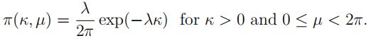
Show that the posterior (marginal) density of κ is
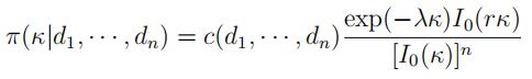
where
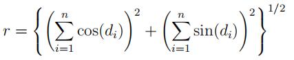
(Hint: To get the marginal posterior density of κ, you need to integrate the joint posterior over µ (from 0 to 2π). The trick is to write
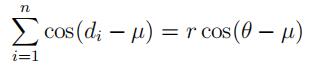
for some θ.)
(c)Thefile txt contains dance
directions of 279 honey bees viewing a zenith patch of artificially polarized light. (The data are given in degrees; you should convert them to radians. The original data were rounded to the nearest 10o; the data in the file have been “jittered” to make them less discrete.) Using these data, compute the posterior density of κ in part (b) for λ = 1 and λ = 0.1. How do these two posterior densities differ? Do these posterior densities “rule out” the possibility that κ = 0 (i.e. a uniform distribution)?Assignment代写
Note: To compute the posterior density, you will need to compute the normalizing constant
– on Quercus, I will give some suggestions on how to do this. A simple estimate of κ is
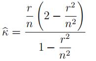
where r is as defined in part (b). The posterior density should be largest for values of κ close to κ; you can use this as a guide to determine for what range of values of κ you should compute the posterior density.
(d)[Bonus] The model that we’ve usedAssignment代写
to this point assumes that κ is strictly positive and thus rules out the case where κ = 0 (which implies that D1, · · , Dnare uniformly distributed). We can actually address the general model (i.e. κ ≥ 0) by putting a prior
probability θ on the model κ = 0 (which implies that we put a prior probability 1 − θ on κ > 0). The prior distribution on the parameter space {(κ, µ) : κ ≥ 0, 0 ≤ µ < 2π} has a point mass of θ at κ = 0 and the prior density over {(κ, µ) : κ > 0, 0 ≤ µ < 2π} is (1 − θ)π(κ, µ). (This is a simple example of a “spike-and-slab” prior, which are used in
Bayesian model selection.) The posterior probability that κ = 0 is then
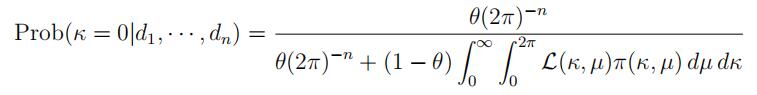
Using the prior π(κ, µ) in part (b) with λ = 1, evaluate Prob(κ = 0|d1, · · · , dn) for θ = 0.1, 0.2, 0.3, · · · , 0.9. (This is easier than it looks as you’ve done much of the work in part (c).)
2.Suppose that F is a continuous distribution with density f .Assignment代写
The mode of the distribution is defined to be the maximizer of the density function. In some applications (for example, when the data are “contaminated” with outliers), the centre of the distribution is better described by the mode than by the mean or median; however, unlike the mean and median, the mode turns out to be a difficult parameter to estimate. There is a document on Quercus thatdiscusses a few of the various methods for estimating the
The τ -shorth is the shortest Assignment代写
interval that contains at least a fraction τ of the observations X1, · · · , Xn; it will have the form [X(a), X(b)] where b − a + 1 ≥ τ n. In this problem, we will consider estimating the mode using the sample mean of values lying in the 1/2-shorth – we will call this estimator the half-shorth-mean. The half-shorth-mean is similar to a trimmed mean but different: For the trimmed mean, we trim the r smallest and r largest observations and average the remaining n − 2r observations; the τ -shorth excludes approximately (1 − τ )n observations but the trimming is not necessarily symmetric.Assignment代写
(a)For the Old Faithful data considered in Assignment #2, compute the half-shorth-mean,usingthe function shorth, which is available on Quercus (in a file txt). Does this estimate make sense?
(b)UsingMonte Carlo simulation, compare the distribution of the half-shorth-mean to that of the sample mean for normally distributed data for sample sizes n = 50, 100, 500, 1000, On Quercus, I have provided some simple code that you may want to modify. We know the variance of the sample mean is σ2/n (where σ2 is the variance of the observations). If we assume that the variance of the half-shorth-mean is approximately a/nγ for some a > 0 and γ > 0, use the results of your simulation to estimate the value of a and γ.
(Hint: If Var(µn) is a Monte Carlo estimate of the variance of the half-shorth-mean for a sample size n, then Assignment代写
ln(Var(µn)) ≈ ln(a) − γ ln(n),
which should allow you to estimate a and γ.)
(c)Itcan be shown that X¯n is independent of µn − X¯n where µn is the half-shorth-mean. (This is a property of the sample mean of the normal distribution – you will learn this in STA452/453.) Show that we can use this fact to estimate the density function of µn from the Monte Carlo data by the “kernel” estimator
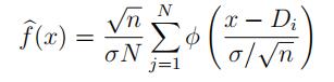
where σ2 = Var(Xi), φ(t) is the N (0, 1) density, and D1, · · · , DN are the values of µn −X¯n from the Monte Carlo simulation. Use the function density (with the approp^riate bandwidth) to give a density estimate for the half-shorth-mean for n = 100.
Supplemental problems (not to hand in):
3.Suppose that X1, · · , Xn Assignment代写
are independent random variables with density or mass func- tion f (x; θ) and suppose that we estimate θ using the maximum likelihood estimator θ; we
estimate its standard error using the observed Fisher information estimator
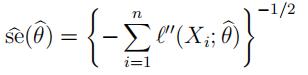
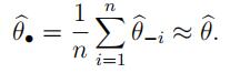
where Aj(x; θ), Ajj(x; θ) are the first two partial derivatives of ln f (x; θ) with respect to θ. Alternatively, we could use the jackknife to estimate the standard error of θ; if our model is correct then we would expect (hope) that the two estimates are similar. In order to investigate this, we need to be able to get a good approximation to the “leave-one-out” estimators {θ−i}.
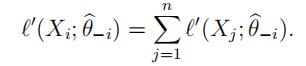
(a)Showthat θ^−i satisfies the equation
(b)Expandthe right hand side in (a), in a Taylor series around θ^ to show that
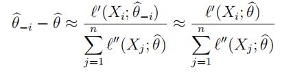
and so
(You should try to think about the magnitude of the approximation error but a rigorous proof is not required.)
(c)Use the results of part Assignment代写
(b) to derive an approximation for the jackknife estimator of the standard error. Comment on the differences between the two estimators – in particular, why is there a difference? (Hint: What type of model – parametric or non-parametric – are we assuming for the two standard errorestimators?)
(d)For the air conditioning data considered in Assignment #1, compute the two standard error estimates for the parameter λ in the Exponential model (f (x; λ) = λ exp(−λx) forx ≥ 0). Do these two estimates tell you anything about how well the Exponential model fits the data?
4.Suppose that X1, · · , Xn
are independent continuous random variables with density f (x; θ) where θ is real-valued. We are often not able to observe the Xi’s exactly rather only if they belong to some region Bk (k = 1, · · · , m); an example of this is interval censoring insurvival analysis where we are unable to observe an exact failure time but know that the failure occurs in some finite time interval. Assignment代写
Intuitively, we should be able to estimate more efficiently with the actual values of {Xi}; in this problem, we will show that this is true (at least) for MLEs.Assume that B1, · · · , Bm are disjoint sets such that P (Xi ∈ ∪m Bk) = 1. Define independent discrete random variables Y1, · · · , Yn where Yi = k if Xi ∈ Bk; the probability mass function of Yi is

Also define
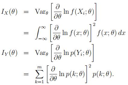
Under the standard MLE regularly conditions, the MLE of θ based on X1, · · · , Xn will have variance approximately 1/{nIX(θ)} while the MLE based on Y1, · · · , Yn will have variance approximately 1/{nIY (θ)}.
(a)Assume the usual regularity conditions for f (x; θ), in particular, that f (x; θ) can be differentiatedwith respect to θ inside integral signs with impunity! Show that IX(θ) ≥ IY (θ) and indicate under what conditions there will be strict
Hints: (i) f (x; θ)/p(k; θ) is a density function on Bk.Assignment代写
(ⅱ)For any functiong,
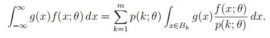
(ⅲ)For anyrandom variable U , E(U 2) ≥ [E(U )]2 with strict inequality unless U is
(b)Underwhat conditions on B1, · · , Bm will IX(θ) ≈ IY (θ)?
5.In seismology,
the Gutenberg-Richter law states that, in a given region, the number of earthquakes N greater than a certain magnitude m satisfies therelationship
log10(N ) = a − b × m
for some constants a and b; the parameter b is called the b-value and characterizes the seismic activity in a region. The Gutenberg-Richter law can be used to predict the probability of large earthquakes although this is a very crude instrument. On Blackboard, there is a file containing earthquakes magnitudes for 433 earthquakes in California of magnitude (rounded to the nearest tenth) of 5.0 and greater from 1932–1992.Assignment代写
(a)If we have earthquakes of (exact) magnitudes M1, · · , Mn
greater than some known m0, the Gutenberg-Richter law suggests that M1, · · · , Mn can be modeled as independent random variables with density
f (x; β) = β exp(−β(x − m0)) for x ≥ m0.
where β = b × ln(10). However, if the magnitudes are rounded to the nearest δ then they are effectively discrete random variables taking values xk = m0 + δ/2 + kδ for k = 0, 1, 2, · · · with probability mass function
p(xk; β) = P (m0 + kδ ≤ M < m0 + (k + 1)δ)
= exp(−βkδ) − exp(−β(k + 1)δ)
= exp(−β(xk − m0 − δ/2)) {1 − exp(−βδ)} for k = 0, 1, 2, · · ·.
If X1, · · · , Xn are the rounded magnitudes, find the MLE of β. (There is a closed-form expression for the MLE in terms of the sample mean of X1, · · · , Xn.)
(b)Compute the MLE of β for the earthquake data (using m0= 4.95 and δ = 0.1) as well
as estimates of its standard error using (i) the Fisher information and (ii) the jackknife. Use these to construct approximate 95% confidence intervals for β. How similar are the intervals?
6.In genetics, Assignment代写
the Hardy-Weinberg equilibrium model characterizes the distributions of genotype frequencies in populations that are not evolving and is a fundamental model of population In particular, for a genetic locus with two alleles A and a, the frequencies of the genotypes AA, Aa, and aa are
Pθ(genotype = AA) = θ2, Pθ(genotype = Aa) = 2θ(1−θ), and Pθ(genotype = aa) = (1−θ)2 where θ, the frequency of the allele A in the population, is unknown.
In a sample of n individuals, suppose we observe XAA = x1, XAa = x2, and Xaa = x3
individuals with genotypes AA, Aa, and aa, respectively. Then the likelihood function is
L(θ) = {θ2}x1 {2θ(1 − θ)}x2 {(1 − θ)2}x3 .
(The likelihood function follows from the fact that we can write Assignment代写
Pθ(genotype = g) = {θ2}I(g=AA){2θ(1 − θ)}I(g=Aa){(1 − θ)2}I(g=aa);
multiplying these together over the n individuals in the sample gives the likelihood function.)
(a)Find the MLE of θ and give an estimator of its standard error using the observed Fisher information.
(b)Auseful family of prior distributions for θ is the Beta family:
where α > 0 and β > 0 are hyperparameters. What is the posterior distribution of θ given XAA = x1, XAa = x2, and Xaa = x3?

更多其他: 物理代写 考试助攻 代写作业 代写加急 代码代写 加拿大代写 北美cs代写 代写CS C++代写 web代写 java代写 数学代写 app代写
