用Python中的LSTM进行股市预测
在Python中发现长期短期记忆(LSTM)网络,以及如何使用它们进行股市预测!
在本教程中,您将看到如何使用称为Long Short-Term Memory的时间序列模型。LSTM模型功能强大,特别是通过设计保留长期记忆,正如您稍后将看到的。您将在本教程中解决以下主题:
-
了解为什么你需要能够预测股票价格走势;
-
下载数据 – 您将使用从雅虎财经收集的股票市场数据;
-
分割列车测试数据并执行一些数据标准化;
-
重新审视并应用一些可用于提前一步预测的平均技术 ;
-
激励并简要讨论LSTM模型,因为它可以预测超过一步;
-
用当前数据预测未来股市并对其进行可视化
如果您不熟悉深度学习或神经网络,请参阅我们的Python深度学习课程。它涵盖了基本知识,以及如何在Keras中自行构建神经网络。这是一个与TensorFlow不同的包,它将在本教程中使用,但这个想法是一样的。
为什么你需要时间序列模型?
你想正确地模拟股票价格,所以作为一个股票买家,你可以合理地决定什么时候买股票,什么时候卖出来赚取利润。这就是时间序列建模的地方。您需要良好的机器学习模型,可以查看数据序列的历史记录,并正确预测序列的未来要素。
警告:股票市场价格非常不可预测且波动很大。这意味着数据中没有一致的模式,可以让您随时间对股价进行近似完美的模拟。不要把它从我这里拿出来,从普林斯顿大学经济学家Burton Malkiel那里拿出来,他在1973年的一本书“随意走下华尔街”中写道,如果市场真的有效率并且股价立即反映所有因素当他们被公开时,被蒙住眼睛的猴子在报纸上市投掷飞镖应该和任何投资专家一样好。
但是,我们不要一直认为这只是一个随机或随机过程,并且机器学习没有希望。让我们看看您是否至少可以对数据进行建模,以便您进行的预测与数据的实际行为相关联。换句话说,你不需要未来的确切股票价值,但股票价格变动(即,如果它在不久的将来会上涨)。
# Make sure that you have all these libaries available to run the code successfullyfrom pandas_datareader import dataimport matplotlib.pyplot as pltimport pandas as pdimport datetime as dtimport urllib.request, jsonimport osimport numpy as npimport tensorflow as tf # This code has been tested with TensorFlow 1.6from sklearn.preprocessing import MinMaxScaler
下载数据
您将使用以下来源的数据:
-
Alpha Vantage。然而,在你开始之前,你首先需要一个API密钥,你可以在这里免费获得。之后,您可以将该键分配给
api_key变量。 -
使用此页面中的数据。您需要将zip文件中的Stocks文件夹复制到项目主文件夹中。
股票价格有几种不同的风格。他们是,
-
开盘价:当天开盘价格
-
关闭:当天的收盘价格
-
高:数据的最高股价
-
低:当日最低股价
从Alphavantage获取数据
您将首先加载来自Alpha Vantage的数据。既然您要利用美国航空股票市场价格做出您的预测,您可以将股票价格设置为"AAL"。此外,您还定义了一个url_string,它将返回一个包含过去20年美国航空所有股票市场数据的JSON文件,以及一个file_to_save将保存数据的文件a 。您将使用ticker您事先定义的变量来帮助命名该文件。
接下来,您将指定一个条件:如果您尚未保存数据,则将继续并从您设置的URL中获取数据url_string; 您将日期,低,高,音量,关闭,开放值存储到熊猫数据框中,df然后将其保存到file_to_save。但是,如果数据已经存在,您只需从CSV中加载它。
从Kaggle获取数据
在Kaggle上发现的数据是csv文件的集合,您不必进行任何预处理,因此您可以直接将数据加载到Pandas DataFrame中。
data_source = 'kaggle' # alphavantage or kaggleif data_source == 'alphavantage':
    # ====================== Loading Data from Alpha Vantage ==================================
    api_key = ''
    # American Airlines stock market prices
    ticker = "AAL"
    # JSON file with all the stock market data for AAL from the last 20 years
    url_string = "https://www.alphavantage.co/query?function=TIME_SERIES_DAILY&symbol=%s&outputsize=full&apikey=%s"%(ticker,api_key)
    # Save data to this file
    file_to_save = 'stock_market_data-%s.csv'%ticker
    # If you haven't already saved data,
    # Go ahead and grab the data from the url
    # And store date, low, high, volume, close, open values to a Pandas DataFrame
    if not os.path.exists(file_to_save):
        with urllib.request.urlopen(url_string) as url:
            data = json.loads(url.read().decode())
            # extract stock market data
            data = data['Time Series (Daily)']
            df = pd.DataFrame(columns=['Date','Low','High','Close','Open'])
            for k,v in data.items():
                date = dt.datetime.strptime(k, '%Y-%m-%d')
                data_row = [date.date(),float(v['3. low']),float(v['2. high']),
                            float(v['4. close']),float(v['1. open'])]
                df.loc[-1,:] = data_row
                df.index = df.index + 1
        print('Data saved to : %s'%file_to_save)
        df.to_csv(file_to_save)
    # If the data is already there, just load it from the CSV
    else:
        print('File already exists. Loading data from CSV')
        df = pd.read_csv(file_to_save)else:
    # ====================== Loading Data from Kaggle ==================================
    # You will be using HP's data. Feel free to experiment with other data.
    # But while doing so, be careful to have a large enough dataset and also pay attention to the data normalization
    df = pd.read_csv(os.path.join('Stocks','hpq.us.txt'),delimiter=',',usecols=['Date','Open','High','Low','Close'])
    print('Loaded data from the Kaggle repository')
Data saved to : stock_market_data-AAL.csv
数据探索
在这里,您将打印收集到DataFrame中的数据。您还应该确保数据按日期排序,因为数据顺序在时间序列建模中至关重要。
# Sort DataFrame by datedf = df.sort_values('Date')# Double check the resultdf.head()
| 日期 | 打开 | 高 | 低 | 关 | |
|---|---|---|---|---|---|
| 0 | 1970年1月2日 | 0.30627 | 0.30627 | 0.30627 | 0.30627 |
| 1 | 1970年1月5日 | 0.30627 | 0.31768 | 0.30627 | 0.31385 |
| 2 | 1970年1月6日 | 0.31385 | 0.31385 | 0.30996 | 0.30996 |
| 3 | 1970年1月7日 | 0.31385 | 0.31385 | 0.31385 | 0.31385 |
| 4 | 1970年1月8日 | 0.31385 | 0.31768 | 0.31385 | 0.31385 |
数据可视化
现在让我们看看你有什么样的数据。您希望随时间发生各种模式的数据。
plt.figure(figsize = (18,9))plt.plot(range(df.shape[0]),(df['Low']+df['High'])/2.0)plt.xticks(range(0,df.shape[0],500),df['Date'].loc[::500],rotation=45)plt.xlabel('Date',fontsize=18)plt.ylabel('Mid Price',fontsize=18)plt.show()

这张图已经说了很多东西。我选择这家公司的具体原因是这张图随着时间的推移出现了不同的股价行为。这将使学习更加强大,并给你一个改变,以测试对于各种情况的预测有多好。
另外需要注意的是,接近2017年的价格要高得多,并且比接近70年代的价格波动更大。因此,您需要确保数据在整个时间范围内的行为相似。在数据标准化阶段,你会处理这个问题。
将数据分成训练集和测试集
您将使用通过获取一天中最高和最低记录价格的平均值计算的中间价格。
# First calculate the mid prices from the highest and lowesthigh_prices = df.loc[:,'High'].as_matrix()low_prices = df.loc[:,'Low'].as_matrix()mid_prices = (high_prices+low_prices)/2.0
现在您可以分割训练数据和测试数据。训练数据将成为时间序列的前11,000个数据点,其余部分将成为测试数据。
train_data = mid_prices[:11000]test_data = mid_prices[11000:]
规范化数据
现在您需要定义一个缩放器来规范数据。MinMaxScalar将所有数据缩放到0和1的范围内。您还可以将训练和测试数据重塑为形状[data_size, num_features]。
# Scale the data to be between 0 and 1# When scaling remember! You normalize both test and train data with respect to training data# Because you are not supposed to have access to test datascaler = MinMaxScaler()train_data = train_data.reshape(-1,1)test_data = test_data.reshape(-1,1)
由于您之前所做的观察,即不同时间段的数据具有不同的值范围,因此您可以通过将整个系列分成多个窗口来标准化数据。如果您不这样做,则较早的数据将接近于0,并且不会为学习过程增加太多价值。在这里你选择一个2500的窗口大小。
提示:在选择窗口大小时,请确保窗口大小不要太小,因为当执行窗口规范化时,它可以在每个窗口的最后引入一个中断,因为每个窗口都是独立标准化的。
在这个例子中,4个数据点会受到这个影响。但是考虑到你有11,000个数据点,4点不会引起任何问题
# Train the Scaler with training data and smooth datasmoothing_window_size = 2500for di in range(0,10000,smoothing_window_size):
    scaler.fit(train_data[di:di+smoothing_window_size,:])
    train_data[di:di+smoothing_window_size,:] = scaler.transform(train_data[di:di+smoothing_window_size,:])# You normalize the last bit of remaining datascaler.fit(train_data[di+smoothing_window_size:,:])train_data[di+smoothing_window_size:,:] = scaler.transform(train_data[di+smoothing_window_size:,:])
将数据重塑为形状 [data_size]
# Reshape both train and test datatrain_data = train_data.reshape(-1)# Normalize test datatest_data = scaler.transform(test_data).reshape(-1)
您现在可以使用指数移动平均数来平滑数据。这有助于您摆脱股票价格数据固有的不规则性并产生更平滑的曲线。
请注意,您只应该平滑训练数据。
# Now perform exponential moving average smoothing# So the data will have a smoother curve than the original ragged dataEMA = 0.0gamma = 0.1for ti in range(11000):
  EMA = gamma*train_data[ti] + (1-gamma)*EMA
  train_data[ti] = EMA# Used for visualization and test purposesall_mid_data = np.concatenate([train_data,test_data],axis=0)
通过求平均的一步预测
平均机制允许您通过将未来股票价格表示为先前观察到的股票价格的平均值来预测(通常是前一步)。这样做多于一个时间步骤可能会产生相当不好的结果。你会看到下面的两种平均技术。标准平均和指数移动平均。您将对两种算法产生的结果进行定性(视觉检测)和定量(均方差)评估。
均方误差(MSE)可以通过取前一步的真值与预测值之间的平方误差并在所有预测中求平均值来计算。
标准平均
您可以首先尝试将此模型作为平均计算问题进行建模,从而了解此问题的难度。首先,您将尝试将未来股票市场价格(例如x t +1)预测为在固定尺寸窗口内的先前观察到的股票市场价格的平均值(例如x t-N,…,x t)(说前100天)。此后,您将尝试更多更漂亮的“指数移动平均线”方法,并看看效果如何。然后你将进入时间序列预测的“圣杯”; 长期短期记忆模型。
首先你会看到正常的平均值是如何工作的。那是你说的,
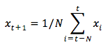
换句话说,你说$ t + 1 $的预测值是你在$ t $到$ tN $窗口内观察到的所有股票价格的平均值。是在t到t–N窗口内观察到的所有股票价格的平均值。t+1tt−N
window_size = 100N = train_data.sizestd_avg_predictions = []std_avg_x = []mse_errors = []for pred_idx in range(window_size,N):
    if pred_idx >= N:
        date = dt.datetime.strptime(k, '%Y-%m-%d').date() + dt.timedelta(days=1)
    else:
        date = df.loc[pred_idx,'Date']
    std_avg_predictions.append(np.mean(train_data[pred_idx-window_size:pred_idx]))
    mse_errors.append((std_avg_predictions[-1]-train_data[pred_idx])**2)
    std_avg_x.append(date)print('MSE error for standard averaging: %.5f'%(0.5*np.mean(mse_errors)))
MSE error for standard averaging: 0.00418
看看下面的平均结果。它紧密地跟踪股票的实际行为。接下来,您将看到更准确的一步预测方法。
plt.figure(figsize = (18,9))plt.plot(range(df.shape[0]),all_mid_data,color='b',label='True')plt.plot(range(window_size,N),std_avg_predictions,color='orange',label='Prediction')#plt.xticks(range(0,df.shape[0],50),df['Date'].loc[::50],rotation=45)plt.xlabel('Date')plt.ylabel('Mid Price')plt.legend(fontsize=18)plt.show()

那么上面的图表(和MSE)会说什么?
对于非常短的预测来说,它似乎并不算太坏(前一天)。鉴于股价在一夜之间不会从0变为100,这种行为是明智的。接下来,您将看到一种称为指数移动平均值的发烧友平均技术。
指数移动平均线
您可能已经在互联网上看到了一些使用非常复杂的模型的文章,并几乎预测了股票市场的确切行为。但要小心!这些只是光学幻想,并不是因为学习有用的东西。您将在下面看到如何使用简单的平均方法来复制该行为。
在指数移动平均法中,您计算$ x_ {t + 1} $ as, as,xt+1
-
X t + 1的 = EMA 吨 =γ×EMA T-1 +(1-γ)x 吨,其中EMA 0 = 0和EMA是你保持随时间的指数移动平均值。
上面的等式基本上是从$ t + 1 $时间步计算出指数移动平均值,并将其用作一步预测。$ \ gamma $决定最近预测对EMA的贡献。例如,$ \ gamma = 0.1 $只能获得EMA当前值的10%。因为你只占最近的一小部分,所以它可以保留你在平均早期看到的更老的值。看看如何用它来预测下面的一步。时间步并将其用作一步预测。γ决定了最近预测对EMA的贡献。例如,γ=0.1只能得到EMA当前值的10%。因为你只占最近的一小部分,所以它可以保留你在平均早期看到的更老的值。看看如何用它来预测下面的一步。t+1γγ=0.1
window_size = 100N = train_data.sizerun_avg_predictions = []run_avg_x = []mse_errors = []running_mean = 0.0run_avg_predictions.append(running_mean)decay = 0.5for pred_idx in range(1,N):
    running_mean = running_mean*decay + (1.0-decay)*train_data[pred_idx-1]
    run_avg_predictions.append(running_mean)
    mse_errors.append((run_avg_predictions[-1]-train_data[pred_idx])**2)
    run_avg_x.append(date)print('MSE error for EMA averaging: %.5f'%(0.5*np.mean(mse_errors)))
MSE error for EMA averaging: 0.00003
plt.figure(figsize = (18,9))plt.plot(range(df.shape[0]),all_mid_data,color='b',label='True')plt.plot(range(0,N),run_avg_predictions,color='orange', label='Prediction')#plt.xticks(range(0,df.shape[0],50),df['Date'].loc[::50],rotation=45)plt.xlabel('Date')plt.ylabel('Mid Price')plt.legend(fontsize=18)plt.show()

如果指数移动平均线很好,为什么你需要更好的模型?
你会发现它符合True分布之后的完美线条(并且由极低的MSE证明)。实际上,仅凭第二天的股票市值就无法做多。个人而言,我想要的不是第二天的确切股票市场价格,但是股票市场价格会在未来30天内上涨或下跌。试着这样做,你会暴露出EMA方法的不可用性。
您现在将尝试在窗口中进行预测(例如,您预测接下来的2天窗口,而不是第二天)。然后你会意识到EMA可能会出错。这里是一个例子:
预测未来一步
为了使事情具体,让我们假设值,例如$ x_t = 0.4 $,$ EMA = 0.5 $和$ \ gamma = 0.5 $xt=0.4EMA=0.5γ=0.5
-
假设你用下面的等式得到输出
-
X t + 1 = EMA t =γ×EMA t-1 +(1-γ)× t
-
所以你有$ x_ {t + 1} = 0.5 \ times 0.5 +(1-0.5)\ times 0.4 = 0.45 $xt+1=0.5×0.5+(1−0.5)×0.4=0.45
-
所以$ x_ {t + 1} = EMA_t = 0.45 $xt+1=EMAt=0.45
-
所以下一个预测$ x_ {t + 2} $变成,xt+2
-
X t + 2 =γ×EMA t +(1-γ)X t + 1
-
它是$ x_ {t + 2} = \ gamma \ times EMA_t +(1 \ gamma)EMA_t = EMA_t $xt+2=γ×EMAt+(1−γ)EMAt=EMAt
-
或者在这个例子中,X t + 2 = X t + 1 = 0.45
因此,无论您预测未来有多少步骤,您都将继续为所有未来的预测步骤获得相同的答案。
你有一个解决方案将输出有用的信息是查看基于动量的算法。他们根据过去最近的价值是上涨还是下跌(而不是确切的价值)做出预测。例如,他们会说如果价格在过去几天一直在下跌,第二天的价格可能会更低,这听起来很合理。但是,您将使用更复杂的模型:LSTM模型。
这些模型已经在时间序列预测领域掀起风暴,因为它们非常擅长建模时间序列数据。您会看到数据中是否存在隐藏的模式,您可以利用这些模式。
LSTMs简介:使股票运动预测未来
长期短期记忆模型是非常强大的时间序列模型。他们可以预测未来的任意步骤。LSTM模块(或单元)具有5个基本组件,可以用它来模拟长期和短期数据。
-
单元状态($ c_t $) – 这表示存储短期记忆和长期记忆的单元的内部记忆ct
-
隐藏状态($ h_t $) – 这是用当前输入计算的输出状态信息,以前的隐藏状态和当前单元格输入,您最终使用它们来预测未来股票市场价格。此外,隐藏状态可以决定仅检索存储在单元状态中的短期或长期或两种类型的存储器以进行下一个预测。ht
-
输入门($ i_t $) – 决定从当前输入流到信元状态的信息量it
-
忘记门($ f_t $) – 决定当前输入和前一个单元状态有多少信息流入当前单元状态ft
-
输出门($ o_t $) – 决定当前单元状态有多少信息流入隐藏状态,因此如果需要,LSTM只能选择长期记忆或短期记忆和长期记忆ot
一个单元格如下图所示。
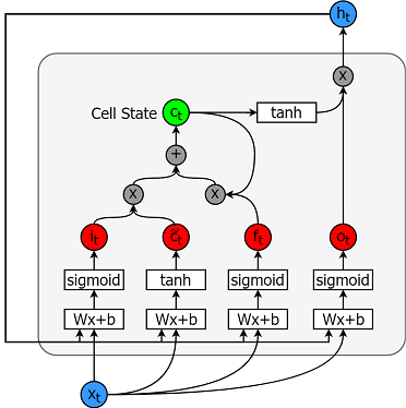
用于计算每个实体的公式如下。
-
$ i t = \ sigma(W {ix} x t + W {ih} h_ {t-1} + b_i)$
-
$ \ tilde {c} t = \ sigma(W {cx} x t + W {ch} h_ {t-1} + b_c)$
-
$ f t = \ sigma(W {fx} x t + W {fh} h_ {t-1} + b_f)$
-
$ c_t = f t c {t-1} + i_t \ tilde {c} _t $
-
$ o t = \ sigma(W {ox} x t + W {oh} h_ {t-1} + b_o)$
-
ht=ottanh(ct)
为了更好地(更技术性)理解LSTM,你可以参考这篇文章。
TensorFlow为实现时间序列模型提供了一个很好的子API(称为RNN API)。你将使用它来实现你的实现。
数据生成器
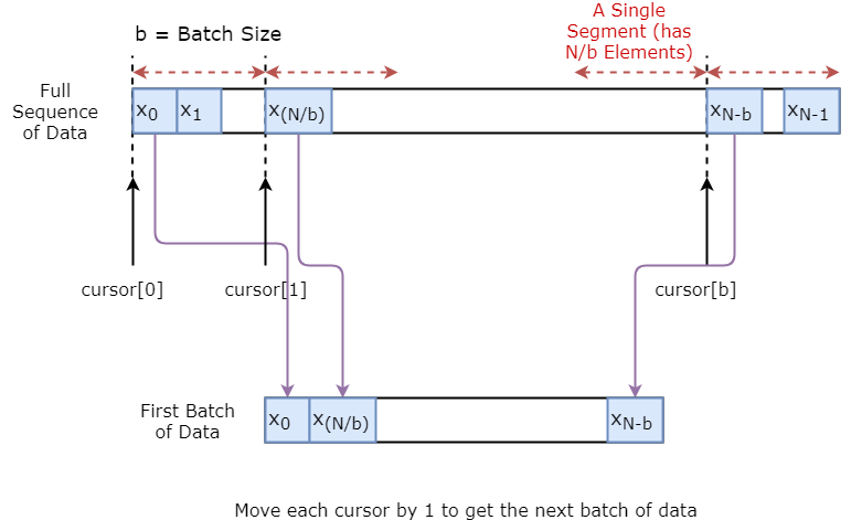
你首先要实现一个数据生成器来训练你的模型。该数据生成器将有一个叫做方法.unroll_batches(...),其将输出一组的num_unrollings依次获得的输入数据,其中,间歇数据的大小是的批次[batch_size, 1]。然后每批输入数据都会有相应的输出批数据。
例如,如果num_unrollings=3和batch_size=4一组展开批次它可能看起来像的,
-
输入数据:$ [x_0,x_10,x_20,x_30],[x_1,x_11,x_21,x_31],[x_2,x_12,x_22,x_32] $[x0,x10,x20,x30],[x1,x11,x21,x31],[x2,x12,x22,x32]
-
输出数据:$ [x_1,x_11,x_21,x_31],[x_2,x_12,x_22,x_32],[x_3,x_13,x_23,x_33] $[x1,x11,x21,x31],[x2,x12,x22,x32],[x3,x13,x23,x33]
数据增强
同样为了使你的模型健壮,你将不会为$ x t $ always $ xalways {t + 1} $ 做出输出。相反,你将随机抽样集合$ x {t + 1},x {t + 2},\ ldots,x_ {t + N} $的输出,其中$ N $是一个小窗口大小。.RatheryouwillrandomlysampleanoutputfromthesetwhereN $是一个小窗口大小。
这里你正在做出以下假设:
-
$ x {t + 1},x {t + 2},\ lots,x_ {t + N} $不会相距太远
我个人认为这是股票运动预测的合理假设。
下面说明如何可视化地创建一批数据。
class DataGeneratorSeq(object):
    def __init__(self,prices,batch_size,num_unroll):
        self._prices = prices
        self._prices_length = len(self._prices) - num_unroll
        self._batch_size = batch_size
        self._num_unroll = num_unroll
        self._segments = self._prices_length //self._batch_size
        self._cursor = [offset * self._segments for offset in range(self._batch_size)]
    def next_batch(self):
        batch_data = np.zeros((self._batch_size),dtype=np.float32)
        batch_labels = np.zeros((self._batch_size),dtype=np.float32)
        for b in range(self._batch_size):
            if self._cursor[b]+1>=self._prices_length:
                #self._cursor[b] = b * self._segments
                self._cursor[b] = np.random.randint(0,(b+1)*self._segments)
            batch_data[b] = self._prices[self._cursor[b]]
            batch_labels[b]= self._prices[self._cursor[b]+np.random.randint(0,5)]
            self._cursor[b] = (self._cursor[b]+1)%self._prices_length
        return batch_data,batch_labels
    def unroll_batches(self):
        unroll_data,unroll_labels = [],[]
        init_data, init_label = None,None
        for ui in range(self._num_unroll):
            data, labels = self.next_batch()
            unroll_data.append(data)
            unroll_labels.append(labels)
        return unroll_data, unroll_labels
    def reset_indices(self):
        for b in range(self._batch_size):
            self._cursor[b] = np.random.randint(0,min((b+1)*self._segments,self._prices_length-1))dg = DataGeneratorSeq(train_data,5,5)u_data, u_labels = dg.unroll_batches()for ui,(dat,lbl) in enumerate(zip(u_data,u_labels)):
    print('\n\nUnrolled index %d'%ui)
    dat_ind = dat
    lbl_ind = lbl
    print('\tInputs: ',dat )
    print('\n\tOutput:',lbl)
Unrolled index 0
    Inputs:  [0.03143791 0.6904868  0.82829314 0.32585657 0.11600105]
    Output: [0.08698314 0.68685144 0.8329321  0.33355275 0.11785509]Unrolled index 1
    Inputs:  [0.06067836 0.6890754  0.8325337  0.32857886 0.11785509]
    Output: [0.15261841 0.68685144 0.8325337  0.33421066 0.12106793]Unrolled index 2
    Inputs:  [0.08698314 0.68685144 0.8329321  0.33078218 0.11946969]
    Output: [0.11098009 0.6848606  0.83387965 0.33421066 0.12106793]Unrolled index 3
    Inputs:  [0.11098009 0.6858036  0.83294916 0.33219692 0.12106793]
    Output: [0.132895   0.6836884  0.83294916 0.33219692 0.12288672]Unrolled index 4
    Inputs:  [0.132895   0.6848606  0.833369   0.33355275 0.12158521]
    Output: [0.15261841 0.6836884  0.83383167 0.33355275 0.12230608]
定义超参数
在本节中,您将定义几个超参数。D是输入的维度。这很简单,因为您将以前的股票价格作为输入,并预测下一个股票的价格1。
那么,你已经知道num_unrollings,这是一个超参数,它涉及用于优化LSTM模型的反向传播时间(BPTT)。这表示您为单个优化步骤考虑了多少个连续时间步骤。您可以将其看作是通过查看单个时间步骤来优化模型,而不是通过查看时间步骤来优化网络num_unrollings。越大越好。
那你就有了batch_size。批量大小是您在单个时间步骤中考虑的数据量。
接下来定义num_nodes哪个表示每个单元中隐藏的神经元的数量。在本例中可以看到有三层LSTM。
D = 1 # Dimensionality of the data. Since your data is 1-D this would be 1num_unrollings = 50 # Number of time steps you look into the future.batch_size = 500 # Number of samples in a batchnum_nodes = [200,200,150] # Number of hidden nodes in each layer of the deep LSTM stack we're usingn_layers = len(num_nodes) # number of layersdropout = 0.2 # dropout amounttf.reset_default_graph() # This is important in case you run this multiple times
定义输入和输出
接下来定义用于培训输入和标签的占位符。这是非常简单的,因为您有一个输入占位符列表,其中每个占位符包含一批数据。该列表中包含num_unrollings占位符,即时用于单个优化步骤。
# Input data.train_inputs, train_outputs = [],[]# You unroll the input over time defining placeholders for each time stepfor ui in range(num_unrollings):
    train_inputs.append(tf.placeholder(tf.float32, shape=[batch_size,D],name='train_inputs_%d'%ui))
    train_outputs.append(tf.placeholder(tf.float32, shape=[batch_size,1], name = 'train_outputs_%d'%ui))
定义LSTM和回归层的参数
你将有三层LSTM和一个线性回归层,用w和表示b,它取得最后一个Long Short Term Memory单元的输出并输出下一个时间步的预测。您可以使用MultiRNNCellTensorFlow封装LSTMCell您创建的三个对象。此外,您可以让Dropout实施LSTM单元,因为它们可以提高性能并减少过度拟合。
lstm_cells = [
    tf.contrib.rnn.LSTMCell(num_units=num_nodes[li],
                            state_is_tuple=True,
                            initializer= tf.contrib.layers.xavier_initializer()
                           )
 for li in range(n_layers)]drop_lstm_cells = [tf.contrib.rnn.DropoutWrapper(
    lstm, input_keep_prob=1.0,output_keep_prob=1.0-dropout, state_keep_prob=1.0-dropout) for lstm in lstm_cells]drop_multi_cell = tf.contrib.rnn.MultiRNNCell(drop_lstm_cells)multi_cell = tf.contrib.rnn.MultiRNNCell(lstm_cells)w = tf.get_variable('w',shape=[num_nodes[-1], 1], initializer=tf.contrib.layers.xavier_initializer())b = tf.get_variable('b',initializer=tf.random_uniform([1],-0.1,0.1))
计算LSTM输出并将其馈送到回归层以获得最终预测
在本节中,您首先创建TensorFlow变量(c和h),它们将保存长短期内存单元的单元状态和隐藏状态。然后,将列表转换train_inputs为具有形状的列表[num_unrollings, batch_size, D],这是计算带有该tf.nn.dynamic_rnn函数的输出所需的。然后使用该tf.nn.dynamic_rnn函数计算LSTM输出,并将输出分解回num_unrolling张量列表。预测与真实股价之间的损失。
# Create cell state and hidden state variables to maintain the state of the LSTMc, h = [],[]initial_state = []for li in range(n_layers):
  c.append(tf.Variable(tf.zeros([batch_size, num_nodes[li]]), trainable=False))
  h.append(tf.Variable(tf.zeros([batch_size, num_nodes[li]]), trainable=False))
  initial_state.append(tf.contrib.rnn.LSTMStateTuple(c[li], h[li]))# Do several tensor transofmations, because the function dynamic_rnn requires the output to be of# a specific format. Read more at: https://www.tensorflow.org/api_docs/python/tf/nn/dynamic_rnnall_inputs = tf.concat([tf.expand_dims(t,0) for t in train_inputs],axis=0)# all_outputs is [seq_length, batch_size, num_nodes]all_lstm_outputs, state = tf.nn.dynamic_rnn(
    drop_multi_cell, all_inputs, initial_state=tuple(initial_state),
    time_major = True, dtype=tf.float32)all_lstm_outputs = tf.reshape(all_lstm_outputs, [batch_size*num_unrollings,num_nodes[-1]])all_outputs = tf.nn.xw_plus_b(all_lstm_outputs,w,b)split_outputs = tf.split(all_outputs,num_unrollings,axis=0)
损失计算和优化器
现在,你会计算损失。但是,您应该注意,计算损失时有一个独特的特征。对于每批预测和真实输出,您可以计算均方误差。你将所有这些均方损失相加(不是平均值)。最后,你定义你将用来优化神经网络的优化器。在这种情况下,您可以使用Adam,它是一个非常新近且性能良好的优化器。
# When calculating the loss you need to be careful about the exact form, because you calculate# loss of all the unrolled steps at the same time# Therefore, take the mean error or each batch and get the sum of that over all the unrolled stepsprint('Defining training Loss')loss = 0.0with tf.control_dependencies([tf.assign(c[li], state[li][0]) for li in range(n_layers)]+
                             [tf.assign(h[li], state[li][1]) for li in range(n_layers)]):
  for ui in range(num_unrollings):
    loss += tf.reduce_mean(0.5*(split_outputs[ui]-train_outputs[ui])**2)print('Learning rate decay operations')global_step = tf.Variable(0, trainable=False)inc_gstep = tf.assign(global_step,global_step + 1)tf_learning_rate = tf.placeholder(shape=None,dtype=tf.float32)tf_min_learning_rate = tf.placeholder(shape=None,dtype=tf.float32)learning_rate = tf.maximum(
    tf.train.exponential_decay(tf_learning_rate, global_step, decay_steps=1, decay_rate=0.5, staircase=True),
    tf_min_learning_rate)# Optimizer.print('TF Optimization operations')optimizer = tf.train.AdamOptimizer(learning_rate)gradients, v = zip(*optimizer.compute_gradients(loss))gradients, _ = tf.clip_by_global_norm(gradients, 5.0)optimizer = optimizer.apply_gradients(
    zip(gradients, v))print('\tAll done')
Defining training LossLearning rate decay operationsTF Optimization operations
    All done
预测相关计算
在这里您可以定义预测相关的TensorFlow操作。首先,在输入(sample_inputs)中定义一个用于馈送的占位符,然后类似于训练阶段,为预测(sample_c和sample_h)定义状态变量。最后,用tf.nn.dynamic_rnn函数计算预测,然后通过回归图层(w和b)发送输出。您还应该定义reset_sample_state重置单元状态和隐藏状态的操作。您应该在开始时执行此操作,每次执行一系列预测。
print('Defining prediction related TF functions')sample_inputs = tf.placeholder(tf.float32, shape=[1,D])# Maintaining LSTM state for prediction stagesample_c, sample_h, initial_sample_state = [],[],[]for li in range(n_layers):
  sample_c.append(tf.Variable(tf.zeros([1, num_nodes[li]]), trainable=False))
  sample_h.append(tf.Variable(tf.zeros([1, num_nodes[li]]), trainable=False))
  initial_sample_state.append(tf.contrib.rnn.LSTMStateTuple(sample_c[li],sample_h[li]))reset_sample_states = tf.group(*[tf.assign(sample_c[li],tf.zeros([1, num_nodes[li]])) for li in range(n_layers)],
                               *[tf.assign(sample_h[li],tf.zeros([1, num_nodes[li]])) for li in range(n_layers)])sample_outputs, sample_state = tf.nn.dynamic_rnn(multi_cell, tf.expand_dims(sample_inputs,0),
                                   initial_state=tuple(initial_sample_state),
                                   time_major = True,
                                   dtype=tf.float32)with tf.control_dependencies([tf.assign(sample_c[li],sample_state[li][0]) for li in range(n_layers)]+
                              [tf.assign(sample_h[li],sample_state[li][1]) for li in range(n_layers)]):
  sample_prediction = tf.nn.xw_plus_b(tf.reshape(sample_outputs,[1,-1]), w, b)print('\tAll done')
Defining prediction related TF functions
    All done
运行LSTM
在这里,您将训练并预测多个时期的股票价格走势,并查看随着时间的推移,预测会变得更好或更糟。您遵循以下过程。
-
定义
test_points_seq时间序列上起点()的测试集以评估模型 -
对于每个时代
-
通过遍历
num_unrollings测试点之前发现的先前数据点来更新LSTM状态 -
n_predict_once使用之前的预测作为当前输入,连续预测步骤 -
计算
n_predict_once预测点与这些时间戳的真实股票价格之间的MSE损失 -
展开一组
num_unrollings批次 -
用展开的批次训练神经网络
-
对于训练数据的完整序列长度
-
计算平均训练损失
-
对于测试集中的每个起点
epochs = 30valid_summary = 1 # Interval you make test predictionsn_predict_once = 50 # Number of steps you continously predict fortrain_seq_length = train_data.size # Full length of the training datatrain_mse_ot = [] # Accumulate Train lossestest_mse_ot = [] # Accumulate Test losspredictions_over_time = [] # Accumulate predictionssession = tf.InteractiveSession()tf.global_variables_initializer().run()# Used for decaying learning rateloss_nondecrease_count = 0loss_nondecrease_threshold = 2 # If the test error hasn't increased in this many steps, decrease learning rateprint('Initialized')average_loss = 0# Define data generatordata_gen = DataGeneratorSeq(train_data,batch_size,num_unrollings)x_axis_seq = []# Points you start your test predictions fromtest_points_seq = np.arange(11000,12000,50).tolist()for ep in range(epochs):
    # ========================= Training =====================================
    for step in range(train_seq_length//batch_size):
        u_data, u_labels = data_gen.unroll_batches()
        feed_dict = {}
        for ui,(dat,lbl) in enumerate(zip(u_data,u_labels)):
            feed_dict[train_inputs[ui]] = dat.reshape(-1,1)
            feed_dict[train_outputs[ui]] = lbl.reshape(-1,1)
        feed_dict.update({tf_learning_rate: 0.0001, tf_min_learning_rate:0.000001})
        _, l = session.run([optimizer, loss], feed_dict=feed_dict)
        average_loss += l
    # ============================ Validation ==============================
    if (ep+1) % valid_summary == 0:
      average_loss = average_loss/(valid_summary*(train_seq_length//batch_size))
      # The average loss
      if (ep+1)%valid_summary==0:
        print('Average loss at step %d: %f' % (ep+1, average_loss))
      train_mse_ot.append(average_loss)
      average_loss = 0 # reset loss
      predictions_seq = []
      mse_test_loss_seq = []
      # ===================== Updating State and Making Predicitons ========================
      for w_i in test_points_seq:
        mse_test_loss = 0.0
        our_predictions = []
        if (ep+1)-valid_summary==0:
          # Only calculate x_axis values in the first validation epoch
          x_axis=[]
        # Feed in the recent past behavior of stock prices
        # to make predictions from that point onwards
        for tr_i in range(w_i-num_unrollings+1,w_i-1):
          current_price = all_mid_data[tr_i]
          feed_dict[sample_inputs] = np.array(current_price).reshape(1,1)
          _ = session.run(sample_prediction,feed_dict=feed_dict)
        feed_dict = {}
        current_price = all_mid_data[w_i-1]
        feed_dict[sample_inputs] = np.array(current_price).reshape(1,1)
        # Make predictions for this many steps
        # Each prediction uses previous prediciton as it's current input
        for pred_i in range(n_predict_once):
          pred = session.run(sample_prediction,feed_dict=feed_dict)
          our_predictions.append(np.asscalar(pred))
          feed_dict[sample_inputs] = np.asarray(pred).reshape(-1,1)
          if (ep+1)-valid_summary==0:
            # Only calculate x_axis values in the first validation epoch
            x_axis.append(w_i+pred_i)
          mse_test_loss += 0.5*(pred-all_mid_data[w_i+pred_i])**2
        session.run(reset_sample_states)
        predictions_seq.append(np.array(our_predictions))
        mse_test_loss /= n_predict_once
        mse_test_loss_seq.append(mse_test_loss)
        if (ep+1)-valid_summary==0:
          x_axis_seq.append(x_axis)
      current_test_mse = np.mean(mse_test_loss_seq)
      # Learning rate decay logic
      if len(test_mse_ot)>0 and current_test_mse > min(test_mse_ot):
          loss_nondecrease_count += 1
      else:
          loss_nondecrease_count = 0
      if loss_nondecrease_count > loss_nondecrease_threshold :
            session.run(inc_gstep)
            loss_nondecrease_count = 0
            print('\tDecreasing learning rate by 0.5')
      test_mse_ot.append(current_test_mse)
      print('\tTest MSE: %.5f'%np.mean(mse_test_loss_seq))
      predictions_over_time.append(predictions_seq)
      print('\tFinished Predictions')
InitializedAverage loss at step 1: 1.703350
    Test MSE: 0.00318
    Finished Predictions
  ...
  ...
  ...Average loss at step 30: 0.033753
    Test MSE: 0.00243
    Finished Predictions
可视化预测
您可以看到MSE损失随着培训的进展而下降。这是模型正在学习有用的东西的好兆头。为了量化您的发现,您可以将网络的MSE损失与您在执行标准平均(0.004)时获得的MSE损失进行比较。你可以看到,LSTM比标准平均做得更好。而且你知道标准平均值(尽管不是完美的)合理地跟随了真实的股价走势。
best_prediction_epoch = 28 # replace this with the epoch that you got the best results when running the plotting codeplt.figure(figsize = (18,18))plt.subplot(2,1,1)plt.plot(range(df.shape[0]),all_mid_data,color='b')# Plotting how the predictions change over time# Plot older predictions with low alpha and newer predictions with high alphastart_alpha = 0.25alpha  = np.arange(start_alpha,1.1,(1.0-start_alpha)/len(predictions_over_time[::3]))for p_i,p in enumerate(predictions_over_time[::3]):
    for xval,yval in zip(x_axis_seq,p):
        plt.plot(xval,yval,color='r',alpha=alpha[p_i])plt.title('Evolution of Test Predictions Over Time',fontsize=18)plt.xlabel('Date',fontsize=18)plt.ylabel('Mid Price',fontsize=18)plt.xlim(11000,12500)plt.subplot(2,1,2)# Predicting the best test prediction you gotplt.plot(range(df.shape[0]),all_mid_data,color='b')for xval,yval in zip(x_axis_seq,predictions_over_time[best_prediction_epoch]):
    plt.plot(xval,yval,color='r')plt.title('Best Test Predictions Over Time',fontsize=18)plt.xlabel('Date',fontsize=18)plt.ylabel('Mid Price',fontsize=18)plt.xlim(11000,12500)plt.show()

虽然不完美,但LSTM似乎能够在大多数时间正确预测股票价格行为。请注意,您正在预测大致在0和1.0的范围内(即不是真实的股票价格)。这是可以的,因为你预测的是股价变动,而不是价格本身。
最后的评论
我希望你发现这个教程很有用。我应该提到,这对我来说是一个有益的经历。在本教程中,我学到了如何设置一个能够正确预测股票价格变动的模型。你开始动机,为什么你需要模拟股票价格。随后是下载数据的说明和代码。然后你看看两种平均技术,可以让你预测未来的一步。您接下来看到,当您需要预测未来的一个以上步骤时,这些方法是徒劳的。此后,您讨论了如何使用LSTM预测未来的许多步骤。最后,你可以看到结果,并看到你的模型(尽管不完美)在正确预测股票价格变动方面非常好。
如果您想深入了解深度学习,请务必查看我们的Python深度学习课程。它涵盖了基本知识,以及如何在Keras中自行构建神经网络。这是一个与TensorFlow不同的包,它将在本教程中使用,但这个想法是一样的。
在这里,我要说明本教程的几个要点。
-
股票价格/运动预测是一项极其困难的任务。就我个人而言,我认为任何股票预测模型都不应该被视为理所当然,并且盲目依赖它们。不过,模型可能能够在大多数时间正确预测股票价格变动,但并非总是如此。
-
不要被那些显示与真实股票价格完美重叠的预测曲线的文章所愚弄。这可以用简单的平均技术来复制,实际上它是无用的。更明智的做法是预测股价走势。
-
模型的超参数对您获得的结果非常敏感。因此,一个很好的做法是在超参数上运行一些超参数优化技术(例如,网格搜索/随机搜索)。下面我列出了一些最重要的超参数
-
优化器的学习率
-
每层中的层数和隐藏单元的数量
-
优化器。我发现亚当表现最好
-
模型的类型。您可以尝试GRU /标准LSTM / LSTM与Peepholes和评估性能差异
-
在本教程中,你做了一些错误的事情(由于数据量很小)!那是你用测试损失来降低学习率。这间接地将关于测试集的信息泄漏到训练过程中。处理这个问题的一个更好的方法是在验证集的性能方面有一个单独的验证集(除了测试集)和衰减学习速率。
如果您想与我联系,可以通过thushv@gmail.com向我发送电子邮件,或者通过LinkedIn与我联系。
参考
我提到这个存储库,以了解如何使用LSTM进行股票预测。但是细节可能与参考文献中的实现大不相同。
