Assignment computer class Risk Theory 2017–2018; week 4
computer class Risk Theory代写 For a certain branch of an insurance company loss ratios were recorded, being the total of the claims
Probability of big loss ratio — Various approximations computer class Risk Theory代写
For a certain branch of an insurance company loss ratios were recorded, being the total of the claims in a week divided by the total earned premium, as a rounded percentage. The total recording period was 100 weeks. Of course big loss ratios are reason for concern. Based on these data, the insurer wants to estimate the probabilities of big and extreme loss ratios, and considers taking a stop-loss like reinsurance to cover the extreme loss ratios.computer class Risk Theory代写
Learning goals of this assignment:
- Useof normal approximation and refinements to estimate probabilities and quantiles
- Graphical display ofdatasets
- Calculating stop-losspremiums
- Censored and truncatedobservations

1 Estimating the cumulants computer class Risk Theory代写
The 100 (rounded) observed loss ratios are stored, not in the order that they occurred but in increasing order,
into vector X like this: computer class Risk Theory代写
X <- scan(text=”
| 68 | 68 | 68 | 69 | 69 | 69 | 69 | 69 | 70 | 70 | 70 | 71 | 71 | 72 | 72 | 72 | 73 | 73 | 73 | 73 |
| 74 | 74 | 74 | 74 | 74 | 75 | 75 | 76computer class Risk Theory代写 | 76 | 76 | 77 | 78 | 78 | 79 | 80 | 80 | 81 | 81 | 81 | 81 |
| 82 | 82 | 82 | 82 | 83 | 83 | 83 | 84 | 84 | 85 | 85 | 87 | 87 | 87 | 89 | 90 | 91 | 91 | 91 | 92 |
| 92 | 92 | 92 | 92 | 93 | 93 | 94 | 95 | 97 | 97 | 97 | 97 | 98 | 98 | 98 | 98 | 99 | 100 | 101 | 101 |
102 102 103 103 104 106 107 108 112 113 116 116 117 126 127 132 132 149 158 170 “)
To be able to use the various approximations, we first have to estimate the first three cumulants of the random variable X of which the numbers given are a sample. They are the mean κ1 = E[X] = µ, the variance κ2 = σ2 = E[(X − µ)2] and the third central moment κ3 = γσ3 = E[(X − µ)3], with γ the skewness.computer class Risk Theory代写
We estimate the population quantities µ, σ and γ simply as follows:
k1 <- mean(X); k2 <- mean((X-k1)^2); k3 <- mean((X-k1)^3); k1; k2; k3 ## 90 381.2 11841.6
With this sample size it does not make a lot of difference if we choose denominator n for the sample variance, such as here, or n − 1, such as in the R-functions var and sd. Such small-sample corrections are applied to give unbiased estimates. But using unbiased estimates for κ2 and κ3 does not mean that γ is estimated without bias. In any case, the simple method- of-moments estimators we use are consistent.
2 A histogram of the data computer class Risk Theory代写
We plot a histogram, and want to add a normal density with as parameters the estimated cumulants k1 and k2 of the sample X.
To combine histogram and fitted density we choose the scale on the y-axis such that the total area of the bars in the histogram is equal to one, by inserting a parameter prob=TRUE. The graphical parameter las=1 produces horizontal labels on the y-axis (see ?par), lwd=2 gives thicker lines, and col=”gray97″ a light-gray color. See colors() to see the possibilities. The fitted density ranges over a wider interval than the data, therefore we let the x-values start at 40, and we ask for (about) 20 breaks in the histogram, leading to bars of width 5. We suppress x and y labels.computer class Risk Theory代写
hist(X, prob=TRUE, col=”gray97″, breaks=20, xlim=c(40,180), las=1, ylim=c(0,.033), yaxp=c(0,.03,3), ylab=””, xlab=””)
curve(dnorm(….), add=TRUE, col=”red”, lwd=2)
Q1 Fill in the dots; see ?curve for how its first parameter should look.computer class Risk Theory代写
Does the random variable X underlying the sample have a normal distribution?
What is the result of the Jarque-Bera test for normality, see Q3 in 18RT1-AppA2EN.pdf?
3 Large loss ratio, normal approximation
Q2 Use the normal approximation to estimate the probability p that the loss ratio is 160% or less. Use a correction for continuity, since the random variable is integer-valued.
If p is the real probability of a value of at most 160%, then calculate the probability of finding a larger value than 160% in a sample of size 100.computer class Risk Theory代写
Do this by filling in the dots in the script below:
y <- (160 + ... - ...)/ ...

p <- pnorm(y)

cat("y =", y, "p =", p, "Probability of 161 or more in sample =", ..., "\n")
4 Large loss ratio, NP-approximation
Judging from the normal approximation, a sample value of more than 160% would be too rare to have reasonably occurred in our sample. Also, the histogram does not look like a normal density, the left-hand tail being too thin.
Q3 Give a more accurate estimate of the probabilities in the previous question by using the NP-method, which accounts for the skewness of the underlying distribution. In gam, store the estimated skewness, in z the argument corrected using the NP-formula, in p the NP- estimated probability of a value 160% or less. Replace the final dots … by the probability of one or more observations being at least 161%.computer class Risk Theory代写
gam <- ...; z <- ...; p <- pnorm(z))

cat("z =", z, "p =", p, "probability of 161 or more in sample =", ...)
From this, is a value of 161% or more still ‘against the odds’ ?
5 Extreme loss ratio, translated gamma approximation computer class Risk Theory代写
In the 100 time periods considered, a loss ratio of over 170% did not occur, but the probability of this event will not be zero. To give a better estimate than the normal approximation, we assume that the unrounded loss ratio X has a translated gamma distribution, that is, X∼ U + x0 with U ∼ gamma(α, β). To estimate the parameters x0, α and β we again assume that the sample values found earlier are equal to the cumulants E[X], Var[X] and E[(X − E[X])3].computer class Risk Theory代写
Q4 In the script below, what has to be filled in to replace the dots to get the probability of a loss ratio of over 170%? See (2.56) and (2.57), or the formulas below Tabel C.For the last line, consult ?pgamma. What is the result of calling the R-functions dgamma, pgamma, qgamma and rgamma? So which of these four do you need here?
mu <- ...; sigma <- ...; gam <- ...

alpha <- ...; beta <- ...; x0 <- ...; y <- ...

1 - ...gamma(y, alpha, beta)
6 Translated gamma approximation in histogram computer class Risk Theory代写
We want to see if the translated gamma approximation fits this dataset better than the normal. We do this, just as above for the normal case, by writing a function to compute the density and adding a plot of it to the histogram.computer class Risk Theory代写
Q5 Fill in the dots, and discuss the result:
dTransGam <- function (x) …gamma(…, alpha, beta) curve(dTransGam(x), add=TRUE, col=”blue”, lwd=2)
7 A ‘stop-loss’ insurance covering extreme loss ratios
To cater for extreme weekly losses, the insurer has found a reinsurer willing to pay b(X −170), with b a certain amount, if the loss ratio X (in %) exceeds 170. To find a premium for thisreinsurance, the corresponding sample quantity will not help, since a loss ratio of this size did not occur up to now. Therefore we use a translated gamma approximation to find a net premium for this stop-loss like reinsurance contract. As an aside, first we give some remarks on the use of a correction for continuity.computer class Risk Theory代写
In the figure on the right, we approximate the discrete cdf F ∼ Uniform({1, 2, 3, 4}) by the continuous cdf G ∼Uniform( 1 , 4 1 ). The cdfs F and G both have mean 2 1 .
For approximating F (k) (• in blue) it seems best to use G(k + 1 ) (∗ in red). In MART (1.33) and Fig. 1.1 you see that the areas of the subsequent triangles between
F and G must cancel. But to approximate the stop-loss premium in e.g. d = 2 with F (the framed gray area, see again MART Fig. 1.1) by the one of G it is better to use argument d = 2 rather than d = 2 1 .
So when approximating stop-loss premiums, it is best not to use the correction for continuity.computer class Risk Theory代写
Q6We already saw that X (≈) U + x with U ∼ gamma(α, β). Formula MART (3.105) com-putes the stop-loss premium of a gamma(α, β) random variable U in d, with G(x; α, β) the gamma(α, β) cdf,
as follows: computer class Risk Theory代写
E[(U − d)+] = 1 − G(d; α + 1, β) − d 1 − G(d; α, β) .
To approximate E[(X − 170)+], which value of d should be taken?
Show that using this formula we get the same result 0.0728876b by integrating the tail 1 − FU (x) of the cdf over (d, ∞) as by computing the stop-loss premium ∫ ∞(x − d)fU (x) dx directly, as predicted by (1.33) in MART.computer class Risk Theory代写
For these last two calculations, write functions sg and xdg to compute the right-hand tail 1 − FU (x) and (x − d)fU (x), respectively, with U ∼ Gamma(α, β):
d <- ...

alpha/beta  *  ... -  d * ... ## MART (3.105)

sg <- function (x) 1-...gamma(...); integrate(...)

xdg <- function(x) (...) * ...gamma(...); integrate(...)
Q7 By (3.101) in MART, for a random variable X with mean µ and variance σ2 we have
![]()
Formulas (3.108) and (3.114) state that by the NP-approximation to the cdf, we have:

Now approximate the stop-loss premium by this technique as well. Your result should not differ more than about 3% from the previous one. Check both if this is not the case.
8 Finding a premium for a reinsurance contract by simulation
In Remark 2.5.8 of MART you find that if U ∼ N(0,1) and γ is ‘small’, a random variable Z = µ + σ U + (U − 1) has mean µ, variance approximately σ and skewness approximately γ. We want to test if this is valid also for the rather large skewness of our sample of loss ratios.
Q8 Generate a sample of size one million from the distribution of Z with µ, σ and γ as estimated from our sample of loss ratios; store it in object XX. Don’t round to integers. Find sample mean, variance and skewness of XX and compare with these estimates. Plot a histogram of XX, with in it normal and translated Gamma approximated curves. Comment.
Q9 We want to set a premium for an insurance that pays an amount b in case the loss ratio is between 140 and 160, 2b if the loss ratio is between 160 and 180, and 3b if it is larger than 180. Estimate the average payment involved from XX. Also compute this premium for a random variable that has the translated Gamma distribution with cumulants as our loss ratio sample.computer class Risk Theory代写
9 Censored and truncated samples computer class Risk Theory代写
In the histograms generated before,
the normal distribution with as parameters sample mean and variance did not fit well over the whole range, because there are no data points below Perhapsthe data were generated by a normal random variable, but the small data simply are missing from the sample, and only the values ≥ 68 were There might be two reasons for this.computer class Risk Theory代写
1.The data are left-truncated. Small values are simply not observed, only large ones, witha threshold of It is not known how many such small values were ignored.
2.The data are left-censored. Small values are only partially known: their exact size is unknown,only that they are less than
Censoring and truncation, both left and right and in combinations, are common in insurance. For instance if there is a retention on an automobile policy, small claims will not be filed. computer class Risk Theory代写If there is a maximum to the insurer’s liability, the part that is not covered is irrelevant, so then there is no need to know the exact value of the damages.
Left-truncated observations computer class Risk Theory代写
First we look at the situation that the data are left- truncated. Assuming the untruncated observations are from a random variable X ∼ N(µ, σ2),our sample is from the conditional distribution of X, given X > 67.5. Actually, the data are rounded to integers, so we sample from |X + 1 ∫, given X > 67.5. Here |x∫ denotes the entier of x, that is, the largest integer ≤ x.
Q10entier of x, that is, the largest integer ≤ x.Write a function that, for its argument x, computes the conditional density of X at x, given X > 67.5. Use again k1, sqrt(k2) as parameters for the normal distribution. Add this function to the plot of Q1.computer class Risk Theory代写
Using the sample mean and s.d. of the truncated sample is clearly not optimal. We will do better by using maximum likelihood estimates, that is, by using the µ, σ2 that maximize the probability of our truncated data. For some X ∼ N(µ, σ2), this probability equals
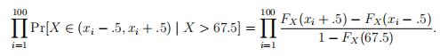
As 1 {F (x + h) − F (x − h)} ≈ F j(x) for small h, the log of the probability of the sample can be approximated by the following function of µ, σ2:
loglik3 <- function(mu.sig)

{-log(prod((dnorm(X,mu.sig[1],mu.sig[2]))/(1-pnorm(67.5,mu.sig[1],mu.sig[2]))))}
Q11 Note that we take the negative because we are going to use optim() to find the parameters giving the maximal likelihood but optim() in its standard mode looks for a minimum. We take the log because we are dealing with very small numbers. Also, instead of two parameters we use a vector of length 2.computer class Risk Theory代写
Write a function loglik2 that computes the exact probability of the sample at parameters mu.sig[1], mu.sig[2]. Compare the results of loglik2 and loglik3 at parameter values mu.sig = c(k1,sqrt(k2)) and mu.sig = c(8,48).computer class Risk Theory代写
Q12 Now do (mu.sig <- optim(c(90,20),loglik3)$par). It can be seen that the ML-estimates
µˆ = 7.65 and σˆ = 47.3 are not at all close to the mean/sd of vector X. We are going to explore this further.
First, investigate if the choice of starting values matters, by trying c(90,20), c(70,30) andc(50,50).
Next, replace loglik3 by loglik2 to see if the exact value gives a different result.
Q13 Under the ML-estimates, find out how many of the observations fall victim to truncating. computer class Risk Theory代写
Q14 We see from Q11 that for the resulting ‘optimal’ parameters, the loglikelihood is indeed larger (≈ −410) than for the sample mean and variance (≈ −426), which maximize the unconditional likelihood. Note that the denominator in the likelihood is about 10−100.Make a plot of the conditional distribution maximizing the likelihood and comment on the fit.
Left-censored observations Now assume that the number of claims that were too small to have been included in the sample is known to be 12. So of 100 data points we know the rounded values given in vector X, of 12 we only know that they were less than 67.5.
Q15 To find the estimates µˆ, σˆmaximizing the probability of our data, write a function giving this probability. It must have one argument mu.sig, which is a vector of length 2, just as before.computer class Risk Theory代写
Then use optim to find the ML-estimates µˆ, σˆ.
To see if the fitted density fits the histogram, extend the data by 4 points equal to 57.5, 8 to62.5. Comment on the fit of the normal density with parameters equal to the ML-estimates of the original sample extended with 12 observations “< 68”.

更多其他: 考试助攻 assignment代写 代写作业 加拿大代写 北美cs代写 代写CS 统计代写 经济代写 计算机代写
