
Problem Set
Advanced Econometrics代写 Please write up your solutions as clearly as possible. Your grade will be reduced if your solution is unreasonably
Advanced Econometrics Part I (Time Series)Advanced Econometrics代写
Please write up your solutions as clearly as possible. Your grade will be reduced if your solution is unreasonably difficult to follow.
Exercise 1:Advanced Econometrics代写
Simulate the series![]() Also generate a time variable. For this exercise, you must attach the do file to your solutions.
Also generate a time variable. For this exercise, you must attach the do file to your solutions.
Data generating process (DGP) for each series is as follows:
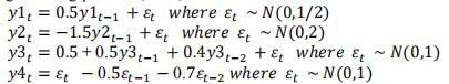
(a) Plot the simulated series on separate graphs
(b) Run 𝑦1𝑡 and 𝑦2𝑡 as an AR(1) model with a drift, save the residuals from this regression and print the histogram of the residuals.
(c)Find the first three autocorrelations and partial autocorrelations, mathematically, foreach of the series Advanced Econometrics代写
(d)Plot the autocorrelations and partial autocorrelations for each of the series aboveand confirm by listing the characteristics of ACs and PACs t
(e) From part (d) can you tell DGP of these series, write an explanation for eachseries separately.
Exercise 2:
A researcher tries to explain the dynamics of 4 global variables: output, inflation, food prices,and oil prices. She could not find evidence for cointegration between the variables.
Hence, she stationarizes and denotes them as {𝑦𝑡, 𝜋𝑡, 𝑓𝑡, 𝑜𝑡}, respectively. She sets up a structural VAR model but could not decide about the restrictions in the structural form matrix.
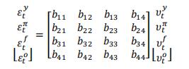
(a) What is the interpretation of 𝑏23?
(b) For identification, what is the minimum number of restrictions the researcher needs?
(c) Based on the economic theory, she thinks the following contemporaneous relationships between the variables hold:
- Output is a slow-moving variable, i.e., other variables cannot affect it, but it can affect others.Advanced Econometrics代写
- Oil prices are essential determinants for both food prices and inflation.
- Food prices cannot affect oil prices, but do affect the inflation.
- The general price level (inflation) is not a determinant for neither oil nor food prices.
Based on the preceding ideas, what kind of restrictions should she put on the structural coefficient matrix, i.e., on bij’s?
(d) Based on the restrictions you have suggested in part (c), explain why she cannot use Choleski identification with this ordering of the variables?
(e) She really wants to use Choleski. Is it possible? Justify your answer.
Exercise 3:
Consider the simple bivariate system of structural VAR:
![]()
(a) Write this system in a standard reduced form; let the error vector in the reduced form to be 𝒆𝑡 . Make sure to show therelation between𝜺𝑡 and 𝒆𝑡.
(b) Simulate the series𝑦1𝑡 , 𝑦2𝑡.For this exercise, you must attach the do file to your solutions.Data generating process (DGP) for each series is as follows:
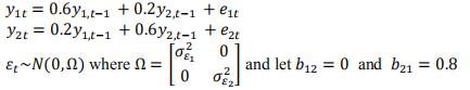
(c) Find the eigenvalues, is this VAR convergent? Why?Advanced Econometrics代写
(d) Find the orthogonolized IRF tables and graphs. Interpret first three steps.
(e) Find FEVD tables. Interpret first three steps.
(f) Now, consider adding one more variable𝑦3
(g) Find the orthogonolized IRF tables and graphs. Interpret first three steps for𝑦3𝑡 only.
(h) Find FEVD tables. Interpret first three steps for 𝑦3𝑡 only.
Exercise 4:
Using housing starts (hs) and 30-year fixed mortgage rate (mrate), given in data set hstarts and mrate.dta
(a)Write the reduced form VAR(1) model in the appropriate form. Discuss if the model is identified. (hint: check Granger causality first). What restriction(s) would you suggest?
(b)Find the orthogonalized impulse response funtions (table only, no need for graphs here),interpret your results.Advanced Econometrics代写
(c) Now, switch the order of the variables in your var command and find the orthogonalized impulse response funtions (table only), interpret your results.
(d)Find forecast error variance decomposition tables, using the order in part (b) interpret your results for the first 3 steps.
(e) (bonus question) Are these series cointegrated, if so run VECM and interpret. If you find them not to be cointegrated explain your reasoning.Advanced Econometrics代写

Exercise 5:
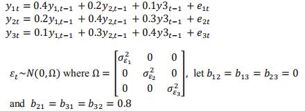
Consider the following VAR(2) model:
![]()
(a) Express𝑦𝑡 as a VAR(1)
(b) Plots the theoretical impulse response function (without using command irf)
(c) Now simulate the data and plot the empirical impulse response function. Is the plot different from the theoretical IRF ?
Exercise 6:
Suppose the residuals of a VAR are such that𝑣𝑎𝑟(𝑒1)= 0.75, 𝑣𝑎𝑟(𝑒2) =0.5 and𝑐𝑜𝑣(𝑒1,𝑒2) =0.25 Advanced Econometrics代写
(a) Show that itis not possible to find the variance matrix of structural VAR shocks from the info given above about the reduced form residual, withoutassuming𝑏12= 0.
(b) Using Cholesky decomposition, find the identified values of 𝑏21, 𝑣𝑎𝑟(𝜀1)and𝑣𝑎𝑟(𝜀2)
Exercise 7:
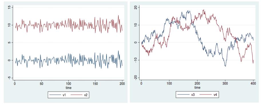
(a) Do variables 𝑣1and𝑣2look cointegrated? Why?
(b) Do variables𝑣3and𝑣4look cointegrated? Why?
(c) Luisahas decided that:
- 𝑣5 and 𝑣6are unit root nonstationary.
- 𝑣5𝑡=0.5𝑣6𝑡 + 𝜀 where 𝜀𝑡 is a stationary variable.
She wants tocon sistentlyes timate a multivariate model. Write out the model in equation/matrix form.Advanced Econometrics代写
(d) Amyhas decided that:
- 𝑣7 and 𝑣8 are unit root nonstationary.
- There does not exist an alpha such that [𝑣7 + 𝛼𝑣8] is stationary.
She wants to consistently estimate a multivariate model. Write out the model in equation/matrix form.
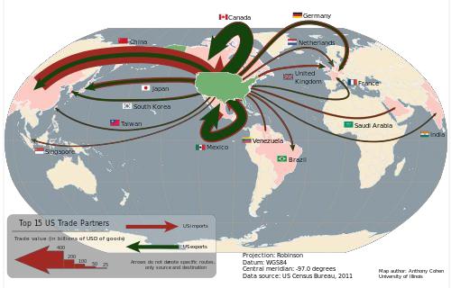
Exercise 8:
For this assignment you will consider top trade partners of US. Use data file named top trade partners.dta, the file exchange rates and interest rates for 5 countries that are top trade partners with US in terms of trade volume. Please write all your commands as a separate do file, you will need to submit the do file with your solutions.
(a) Graph all exchange rate series on 5 separate graphs at once (using combine graph command) copy/paste all graphs on your answer sheet.
(b) Graph all interest rates series on 5 separate graphs at once (using combine graph command) copy/paste all graphs on your answer sheet.
(c) Check for cointegration and run the most appropriate VAR or VECM model (note that you may need to set matsize 450 before you can run some of the commands you need)Advanced Econometrics代写
(d) Using the model in part (c) forecast exchange rates (let the dynamic forecast start in February 2014 and end in July 2014). List results and interval for Canada and Europe,graph forecast and interval for Mexico and China (list and graph should start on December 2013.
(e) Run a multivariate GARCH(1, 1) model with constant conditional correlation, for interest rates in Canada, European Union and Mexico. Write your results in equation form.
Exercise 9:
For this exercise convert the data in exercise 8 into panel form.
(a) Run fixed effects model regressing exchange rate on interest rate. What does fixed effects model control for? How? Interpret your results.
(b) Run between effects model regressing exchange rate on interest rate. What does between effects model control for? How? Interpret your results.
(c) Run random effects model regressing exchange rate on interest rate. Explain this model,why would a researcher prefer to use random effects model here? Interpret your results.Advanced Econometrics代写
(d) Apply Hausman test, interpret the results, which model is more reliable according to Hausman test?
(e) How would you go about estimating a dynamic panel model?
Exercise 10:
This problem set asks you to run recursive vector autoregressions (VAR) similar to those discussed in Stock and Watson (2001)1 and consider the robustness of the estimates that these VARs yields along several dimensions. You are free to use whichever statistical/computational package you would like. But I recommend that you use Stata both because it is relatively simple to do what I ask for in Stata and because having a facility with Stata is extremely useful for you going forward. Please hand in a writeup with the results we ask for below and also your code.Advanced Econometrics代写
(a) Baseline VAR:
i.Download quarterly data on the U.S. GDP deflator and U.S. real GDP, and monthly data on the the federal funds rate from 1960 to the present. Construct an inflation rate as 𝜋𝑡 = 400𝑙𝑛(𝑃𝑡/𝑃𝑡−1 ), where𝑃𝑡 is the GDP deflator. Construct a growth rate for realGDP as ∆𝑌𝑡= 400 ln(𝑌𝑡/𝑌𝑡−1 ), where𝑌𝑡 is real GDP. Construct a quarterly series for the federal funds rate by averaging the monthly values within quarter.
ii.Estimate a recursive VAR using these three variables ordered: 1) inflation, 2) GDP growth, 3) interest rate. Or equivalently, estimate a reduced form VAR of these three variables and compute the Cholesky factorization of the reduced form VAR covariance matrix. Use four lags in your VAR. Use the sample period 1960:I-2016:IV.
iii. Calculate impulse response functions of the three variables to the monetary policy shock from this VAR (i.e., the shock in the interest rate equation). Plot the point estimates along with estimates of 95% asymptotic confidence intervals. Plot each impulse response separately, or otherwise adjust the axes in such a way to make sure that each one is clearly visible. Plot the impulse response functions for 20 quarters.
iv.Briefly describe these impulse responses and what they imply about the effects of monetary policy.Advanced Econometrics代写
1 Stock, J. H. and M. W. Watson (2001) “Vector Autoregressions,” Journal of Economic Perspectives, 15(4), 101–115.
v.Calculate the forecast error variance decomposition of all three variables due to the monetary policy shock at horizons of 1, 8 and 20 quarters.
vi.Briefly comment on these results.
(b) An important concern when interpreting the output of VARs is the possibility of omitted variables bias.
Let’s now add one additional variable to our VAR and see if this affects the conclusions we come to
i.Download the ISM Manufacturing: Purchasing Manager Index (PMI) Composite Index from the Fred database at the St. Louis Federal Reserve (Data source: https://www.quandl.com/data/FRED/NAPM-ISM-Manufacturing-PMI-Composite-Index 2). This index is based on a survey of purchasing managers in the manufacturing sector and attempts to gauge the state of this sector. It is constructed from five sub-indexes on production levels, new orders, supplier deliveries, inventories and employment levels. This index is considered a leading indicator for the economy. Construct a quarterly series from the monthly data by averaging within quarter.Advanced Econometrics代写
ii.Estimate a recursive VAR using the four variables you have downloaded ordered: 1)inflation, 2) GDP growth, 3) ISM index 4) interest rate. Or equivalently, estimate are duced form VAR of these four variables and compute the Cholesky factorization of the reduced form VAR covariance matrix. Use four lags in your VAR. Use the sample period 1960:I-2007:IV.
iii. Calculate impulse response functions of inflation, growth, and the interest rate to the monetary policy shock from this VAR. Briefly describe these impulse responses, how they compare to the impulse responses for the baseline VAR, and what may explain why they differ from the impulse responses in the baseline VAR. You may find it useful to also calculate the cumulative impulse responses of inflation and output growth, i.e., the responses of the price level and the level of output, in assessing the sensitivity of the results to the inclusion of the ISM index.
iv.Calculate the forecast error variance decomposition of all three variables due to the monetary policy shock at horizons of 1, 8 and 20 quarters. Briefly comment on these results and compare them to the corresponding results for the baseline VAR.
(c) It is interesting to consider whether the results we get are sensitive to the sample period used.In particular,
some have argued that the conduce of monetary policy changed dramatically when Paul Volcker took over as chairman of the Federal Reserve in October 1979.
i.Reestimate the VAR you estimated in part A for two sub-samples: 1) 1960:I-1979:III,and 2) 1979:IV-2016:IV Advanced Econometrics代写
ii.Calculate impulse response functions of the three variables to the monetary policy shock from this VAR. Briefly describe these impulse responses, how they compare, and what they imply about the results from part A.
iii. Calculate the forecast error variance decomposition of all three variables due to the monetary policy shock at horizons of 1, 8 and 20 quarters for these two subsample.Briefly comment on these results, how they compare, and how they compare to the corresponding results for the VAR estimated in part A.
2 To download data, you need to create a free student account first.
更多其他:C++代写 r代写 考试助攻 C语言代写 finance代写 lab代写 计算机代写 code代写 report代写 project代写 物理代写 数学代写 java作业代写 经济代写
