
The Sustainable Black-Scholes Equations
Black-Scholes Equations代写 In incomplete markets, a basic Black-Scholes perspective has to be complemented by the valuation
Yannick Armenti1 St´ephane Cr´epey1 Chao Zhou2
AbstractBlack-Scholes Equations代写
In incomplete markets, a basic Black-Scholes perspective has to be complemented by the valuation of market imperfections. Otherwise this results in Black-Scholes Ponzi schemes, such as the ones at the core of the last global financial crisis, where always more derivatives need to be issued for remunerating the capital attracted by the already opened positions. In this paper we consider the sustainable Black-Scholes equations thatarise for a portfolio of options if one adds to their trade additive Black-Scholes price, on top of a nonlinear funding cost, the cost of remunerating at a hurdle rate the residual risk left by imperfect hedging. We assess the impact of model uncertainty in this setup.
Keywords: Market incompleteness, cost of capital (KVA), cost of funding (FVA), model risk, volatility uncertainty, optimal martingale transport.
1 IntroductionBlack-Scholes Equations代写
In incomplete markets, a basic Black-Scholes perspective has to be complemented by the valuation of market imperfections. Otherwise this results in Black-Scholes Ponzi schemes,such as the ones at the core of the last global financial crisis, where always more derivativesneed to be issued for remunerating the capital attracted by the already opened positions. In this paper we consider the sustainable Black-Scholes equations that arise for a portfolio ofoptions if one adds to their trade additive BlackScholes price, on top of a nonlinear funding cost, the cost of remunerating at a hurdle rate the residual risk left by imperfect hedging. We assess the impact of model uncertainty in this setup.
Section 2 revisits the pricing of a book of options accounting for cost of capital and cost of funding,
which are material in incomplete markets. Section 3 specializes the pricing equations to a Markovian Black–Scholes setup. Section 4 assesses the impact of model risk in an UVM (uncertain volatility model) setup. Section 5 refines the model risk add-ons by accounting for calibrability constraints.Black-Scholes Equations代写
We consider a portfolio of options made of ωi vanilla call options of maturity Ti and strike Ki on a stock S, with 0 < T1 < . . . < Tn = T. Note that, if a corporate holds a bankpayable, it typically has an appetite to close it, receive cash, and restructure the hedgeotherwise with a par contract (the bank would agree to close the deal as a market maker,
1 University of Evry Val d’Essonne, Evry, France
2 Department of Mathematics, National University of Singapore, Singapore, matzc@nus.edu.sg.Black-Scholes Equations代写
Acknowledgement: The research of St´ephane Cr´epey benefited from the support of the “Chair Markets in Transition”, F´ed´eration Bancaire Franc¸aise, of the ANR project 11-LABX-0019 and of the EIF grant “Collateral management in centrally cleared trading”. The travel expenses of St´ephane Cr´epey regarding its participation to the ICASQF 2016 conference were funded by l’Institut Franc¸ais de Colombie, Carrera 11 No. 93-12, Ambassade de France en Colombie. The research of Chao Zhou is supported by NUS Grants R-146-000-179-133 and R-146-000-219-112.Black-Scholes Equations代写
charging fees for the new trade). Because of this natural selection, a bank is mostly in the receivables (i.e. “ωi ≥ 0”) in its derivative business with corporates.
We write x± = max(±x, 0).

2 Cost of Capital and Cost of FundingBlack-Scholes Equations代写
2.1 Cost of Capital
In presence of hedging imperfections resulting in a nonvanishing loss (and profit) process ̺ of the bank, a conditional risk measure EC = ECt(̺) must be dynamically computed and reserved by the bank as economic capital.Black-Scholes Equations代写
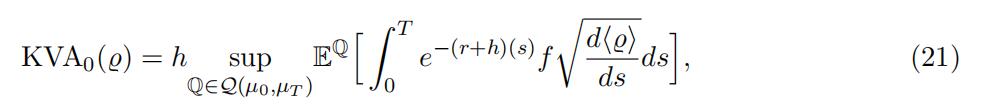
It is established in Albanese, Caenazzo, and Cr´epey (2016, Section 5) that the capital valuation adjustment (KVA) needed by the bank in order to remunerate its shareholders for their capital at risk at some average hurdle rate h (e.g. 10%) at any point in time in the future is:
KVA = KVAt(̺) = hEtTe−(r+h)(s−t)tECs(̺)ds, (1)Black-Scholes Equations代写
where Et stands for the conditional expectation with respect to some probability measure Q and model filtration.
In principle, the probability measure used in capital and cost of capital calculations should be the historical probability measure. But, in the present context of optimization of a portfolio of derivatives, the historical probability measure is hard to estimate in a relevant way, especially for long maturities. As a consequence, we do all our price and risk computations under a risk-neutral measure Q calibrated to the market (or a family of pricing measures, in the context of model uncertainty later below), assuming no arbitrage.
2.2 Cost of FundingBlack-Scholes Equations代写
Let rt denote a risk-free OIS short term interest rate and βt = e− , rsds be the correspondingtrisk-neutral discount factor. We assume that the bank can invest at the risk-free rate r but can only obtain unsecured funding at a shifted rate r + λ > r. This entails funding costsover OIS and a related funding valuation adjustment (FVA) for the bank.Black-Scholes Equations代写
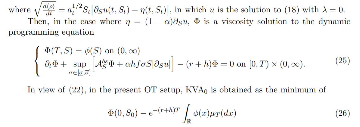
Given our focuson capital and funding in this paper, we ignore counterparty risk for simplicity, so that λ isinterpreted as a pure funding liquidity basis. In order to exclude arbitrages in the primarymarket of hedging instruments, we assume that the vector gain process M of unit positions held in the hedging assets is a risk-neutral martingale. The bank “marks to the model”its derivative portfolio, assumed bought from the client at time 0, by means of an FVA- deducted value process Θ.
The bank may also set up a (possibly imperfect) hedge (−η) in the hedging assets,
for some predictable row-vector process η of the same dimension asM.Weassume that the depreciation of Θ, the funding expenditures and the loss ηdMon the hedge, minus the option payoffs as they mature, are instantaneously realized intothe loss(-and-profit) process ̺ of the bank. In particular, at any time t, the amount on the funding account of the bank is Θt. Moreover, we assume that the economic capital can be used by the trader for her funding purposes provided she pays to the shareholders the OIS rate on EC that they would make otherwise by depositing it (assuming it all cash for simplicity).Black-Scholes Equations代写
Note that the value process Θ of the trade already includes the FVA as a deduction,
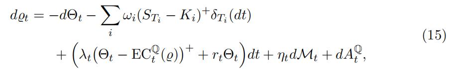
but ignores the KVA, which is considered as a risk adjustment computed in a second step (in other words, we assume that the trader’s account and the KVA account are kept separate from each other). Rephrasing in mathematical terms the above description, the loss equation of the trader is written, for t ∈ (0, T ], as (starting from ̺0 = y, the accrued loss of the portfolio):
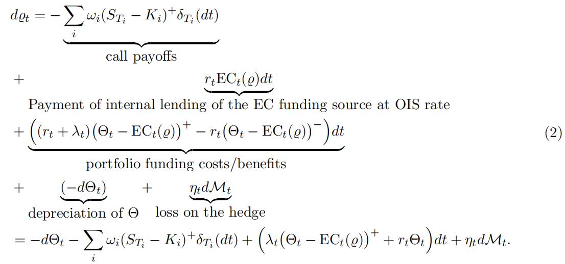
Hence, a no-arbitrage condition that the loss process ̺ of the bank should follow a risk-neutral martingale (assuming integrability) and the terminal condition ΘT = 0 lead to the following FVA-deducted risk-neutral valuation BSDE:
(since we consider a portfolio of options with several maturities, we treat option pay-offs as cash-flows at their maturity times rather than a terminal condition in the equations, in particular ΘT = 0).
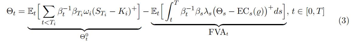
The funding source provided by economic capital creates a feedback loop from EC into FVA, which makes the FVA smaller.
Note that, in the usual case of a risk measure EC only affected by the time fluctuationsof ̺, the equations (3) and in turn (1) are independent of the accrued loss y, which eventually does not affect Θ nor the KVA.Black-Scholes Equations代写
If λ = 0, then, whatever the hedge η, Θ reduces to Θ0, which corresponds to the usual
trade additive (linear) no-arbitrage pricing formula for a portfolio of options, with zero FVA, but with a KVA given by (1), depending on the hedge η.
If λ 0, we introduce the following backward SDE:

This is a monotone driver backward SDE, admitting as such a unique square integrable solution Θ⋆ (see e.g. Kruse and Popier (2016, Sect. 4)), provided λ is bounded from belowand Θ0 is square integrable. If there exists a replicating hedge η, i.e. η = η⋆ such that the corresponding ̺ is constant in (2), i.e. η⋆dMt coincides with the martingale part of Θ⋆,then the resulting ̺, EC and KVA vanish (since we assumed EC(0) = 0) and the ensuing FVA-deducted value process is given by Θ⋆.
Example 2.1 (Single option positions) If n = 1 and ω1 = 1 (one long call position),
then, by application of the comparison theorem for BSDEs with a monotonic generator (see Kruse and Popier (2016, Sect. 4)), we have Θ⋆ ≥ 0, hence
Θ⋆ = EtΣβ˜−1β˜T (ST − K1)+Σ, (5)
where eβt =e− Rt0(r+λs)ds . With respect to Θ(0), the value Θ⋆ corresponds to an FVA rebate on the buying price by the bank (since we assumed a positive liquidity basis λ).Black-Scholes Equations代写
If n = ω1 = 1 (one short call position), then we deduce likewise that Θ⋆ 0, hence Θ⋆ = Θ(0).
But, apart from the above special cases where λ = 0 or η = η⋆, the BSDE (3) for Θ is nonstandard due to the term EC = ECt(̺) in the FVA.
3 Markovian Black-Scholes SetupBlack-Scholes Equations代写
In this section we assume a constant risk-free rate r and a Black-Scholes stock S with volatility σ and constant dividend yield q. The risk-neutral martingale M is then taken as the gain process of a continuously rolled unit position on the stock S, assumed funded at the risk-free rate via a repo market, i.e. dMt = dSt − (r − q)Stdt. We denote by
Abs = (r − q)S∂S + 1 σ2S2∂22 the corresponding risk-neutral Black-Scholes generator.
Doing our modeling exercise in the context of the Black-Scholes model, where perfect replication, hence no KVA, is possible, may seem rather artificial. However, doing all the computations in a stylized Black-Scholes setup with a single risk factor S yields useful prac- tical insights.Black-Scholes Equations代写
In addition, this conveys the message that, in real-life incomplete markets, a basic Black-Scholes perspective has to be complemented by the valuation of market im- perfections, otherwise this unavoidably results in Black-Scholes Ponzi schemes, such as the ones that have been involved in the global financial crisis, where always more derivatives are issued to remunerate the capital required by the already opened positions (if priced and risk-managed in a basic Black-Scholes way ignoring the cost of capital).
In the Black-Scholes setup and assuming a stylized Markovian specification
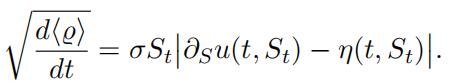
EC (̺) = f . d (̺)(6)
(the stylized VaR which is proportional to the instantaneous volatility of the loss process ̺ modulo a suitable “quantile level” f ) as well as λ = λ(t, St), ηt = η(t, St), then the above FVA and KVA equations can be reduced to the “sustainable Black-Scholes PDEs” (12), as Black-Scholes Equations代写
follows (resulting in an FVA- and KVA-deducted price that would be sustainable for the bank even in the limit case of a portfolio held on a run-off basis, with no new trades ever entered in the future).
First, observe that given a tentative FVA-deducted price process of the form Θt =
u(t, St) for some to-be-determined function u = u(t, S), we have, assuming (6):
(7)
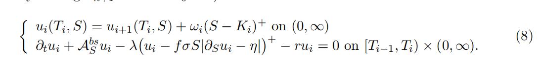
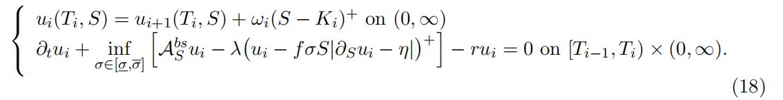
Accordingly, let the function u be defined by ui(t, S) on each strip (Ti−1, Ti] × (0, ∞),
where (ui)1≤i≤n is the unique sequence of viscosity solutions, which can then shown to be classical solutions, to the following PDE cascade, for i decreasing from n to 1 (closing the system by setting un+1 = 0 and T0 = 0):Black-Scholes Equations代写
Itoˆ calculus shows that the process Θ = (u(t, St))t solves the Markovian, monotonic driver (assuming λ bounded from below) BSDE
which in view of (6)-(7) is precisely (3).
The ensuing FVA= Θ(0) − Θ and KVA processes are given as (cf. (3) and (1)):
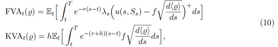
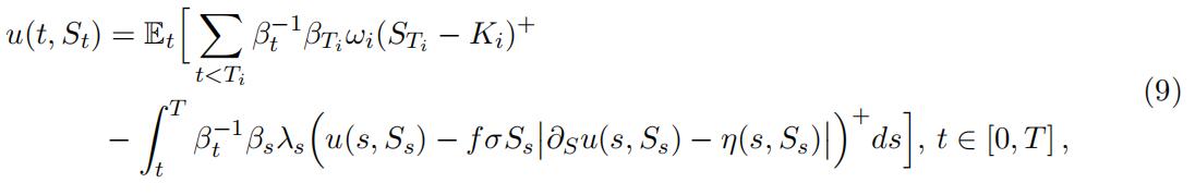
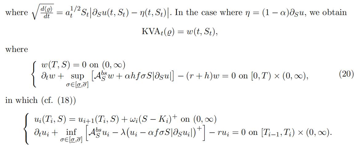
where d (̺) is given by (7). We set η = (1 − α)∂Su, where α in [0, 100%] is the mis-hedge parameter (noting that, for α = 0, the BSDE (9) reduces to the replication BSDE (4)), then the latter reduces to ασSt.∂Su(t, St). and we have
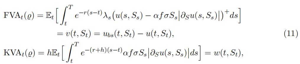
where ubs is the trade additive Black-Scholes portfolio value and where the FVA and KVA pricing functions v and w satisfy
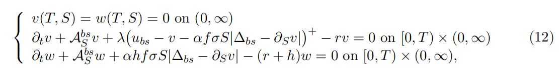
These “sustainable Black-Scholes PDEs” (12) allow computing an FVA and KVA de-
ducted price
u − w = ubs − v − w
that would be sustainable for the bank even in the limit case of a portfolio held on a run-off basis, with no new trades ever entered in the future.
4 With Volatility Uncertainty Black-Scholes Equations代写
An important and topical issue, referred to by the regulation as AVA (additional valuation adjustment), is the magnifying impact of model risk on the different XVA metrics.
In this section, we assess model risk from the angle of Avellaneda, Levy, and Paras (1995)’s uncertain volatility model (UVM). Namely, we only assume positive bounds σ and σ but we do not assume any specific dynamic on the stock volatility process σ. Therefore,there is a model uncertainty about it. That is, we only consider dMt := σtStdWt =dSt − (r − q)Stdt, where σt ∈ [σ, σ] for every t.
We call C the space of continuous paths on R+,
C the canonical process on the space C, F = (Ft)0≤t≤T the canonical filtration generated by C and Q the set of F local martingale probability measures for C. We recall from Soner, Touzi, and Zhang (2012) that, for any probability measure Q ∈ Q, the process C satisfies dCt = a1/2dW Q, for some Q Brownian motion W Q, where at is the Lebesgue density of the aggregated quadratic variation of C. In the following we restrict attention to the probability measures Q such that a1/2 ∈ [σ , σ] holds dt × Q almost surely, still denoting by Q the (restricted) set of measures, and we model dMt = dSt − (r − q)Stdt as StdCt.Black-Scholes Equations代写
Under each Q, similarly to (2), the loss equation of the trader is written, for t ∈ (0, T ],as:

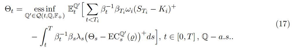
where ECQ is some conditional risk measure under Q. The ensuing equation for the Q FVA-deducted value ΘQ appears as

Under each Q, the trader should value the derivative portfolio ΘQ at time 0 (or ΘQ 0 t at time t). However, due to the model uncertainty, the trader values it Θ0 = inf ΘQ (orQ∈Q 0 at time t, Θt = ess inf ΘQ), which is a robust non-arbitrage price in the sense of (Biagini,Q∈Q Bouchard, Kardaras, and Nutz 2015).
At time t, ECQ(̺Q) may depend on the whole future of the process (̺Q), s ≥ t. This
makes (14) a so-called anticipated BSDE under Q (ABSDE in the sense of Peng and Yang(2009)), with generator λt.ΘQ − ECQ(̺Q)Σ+, where ΘQ corresponds to the “Y -component”and (d̺Q ηsSsdCs) to the “Z-component” of the solution. However, in the Markoviansetting of Sect. 3, ECQ(̺Q) only depends on (̺Q) at time t, so that the ABSDE (14)t treduces to a BSDE.Black-Scholes Equations代写
For taking model risk (i.e. the impact of several Q) into consideration, we need the notion of second order BSDE. Wellposedness results regarding second order anticipated BSDEs are not yet available in the literature. Hence, we only give heuristic formulations in this regard. Namely, by analogy with the second order BSDEs theory introduced by
Soner, Touzi, and Zhang (2012), we should have the following representation, where F+ = (F+)0≤t≤T the right limit of F, i.e. F+ = ∩s>tFs for all t ∈ [0, T ) and F+ = FT :
There exists a process ̺ such that, for each Q ∈ Q, ̺ is a Q-local martingale
and it Q − a.s. holds thatBlack-Scholes Equations代写
where ECQ is some conditional risk measure and the family {AQ} of non- decreasing processes satisfies the minimality condition
AQ = ess infQ EQ′ Σ AQ′ . FQ+Σ , 0 ≤ t ≤ T, Q − a.s., ∀Q ∈ Q, (16)
where Q(t, Q, F+) := Q′ ∈ Q, Q′ = Q on F+ .
The corresponding equation for the FVA-deducted value Θ would appear as
4.1 Equations in the Markovian SettingBlack-Scholes Equations代写
By contrast, in the Markovian setting of Sect. 3 with VaR-like specification of Economic Capital, we can make rigorous statements. According to the second order BSDE theory introduced in Soner, Touzi, and Zhang (2012), the PDE (8) becomes:
Let u be defined by ui(t, S) on each strip (Ti−1, Ti] × (0, ∞). The FVA can be defined as Θλ=0 − Θ and the ensuing KVA process is given as (cf. (3) and (1)):

5 Optimal Transportation Approach
Since vanilla call options are liquidly traded, their time 0 price components
EQΣβTi (STi − Ki)+Σ
should not be seen as subject to model risk, but calibrated to the market. Hence, we need to refine our preliminary UVM assessment of model risk in order to account for these calibration constraints. For simplicity we consider a single call option (T, K) and we set λ = 0, focusing on KVA in this section. Hence, the system (18) reduces to a single PDE with λ = 0, with solution denoted by u.
(Tan and Touzi (2013))
consider the optimal transportation problem consisting of minimizing a cost among all continuous semimartingales with given initial and terminal distri- butions. They show an extension of the Kantorovitch duality to this context and suggest a finite-difference scheme combined with the gradient projection algorithm to approximate the dual value. Their results can be applied to our setup as follows.
Let µ0 = δS0 denote the Dirac measure on the initial value of S0 and let µT denote the marginal distribution of ST , inferred by calibration to the market prices of all European call options with maturity T (assuming quotations available for all strikes). Let
Q(µ0) = {Q ∈ Q : Q ◦ S0−1 = µ0}, Q(µ0, µT ) = {Q ∈ Q(µ0) : Q ◦ S−1 = µT }.Black-Scholes Equations代写
From the remark 2.3 in Tan and Touzi (2013), Q(µ0, µT ) is not empty in our setting.
The KVA with model uncertainty and terminal marginal constraint is defined as fol-
lows:
where ̺ represents the portfolio loss in this setting, that is, the loss and profit of the bank in a world with uncertain volatility subject to the law of ST . However, it is not clear how to extrapolate the theory of Tan and Touzi (2013) to valuation at future time points when only the unconditional law of ST is known. Hence for the sake of tractability we conservativelyassume that ̺ in (21) is the UVM one and we only apply the constraint to the outerexpectation in (21) (as opposed to the conditional expectations that are hidden in ̺).
With this understanding of (21), given any measure ν, we define
ν(φ) = ∫R φ(x)ν(dx)Black-Scholes Equations代写
on the set Cb(Rd) of all bounded continuous functions φ on Rd. We can readily check that Assumptions 3.1-3.3 in Tan and Touzi (2013) are satisfied. Hence, by an application of their main duality result, we can rewrite the KVA as

where the “pseudo-payoff function” φ corresponds to a Lagrangian for the constrained optimization problem (21) and where

Hence, the KVA in an optimal transportation (OT) setting can be represented as an infimum of KVAs in modified UVM setting.Black-Scholes Equations代写
5.1 Equations in the Markovian Setting
In the Markovian setting of Sect. 3, we consider the probability measures Q on the canonical space (Ω, FT ), under which the canonical process C is a local martingale on [t, T ]. DefineQt as the collection of all such martingale probability measures Q such that as ∈ [ σ, σ] dQ × ds–a.e. on Ω × [t, T ]. Denote Qt,x := {Q ∈ Qt : Q[Ss = x, 0 ≤ s ≤ t] = 1}. For any φ ∈ Cb(Rd), let

over φ ∈ Cb(Rd). This minimization is achieved numerically by the Nelder-Mead simplex algorithm.
As a sanity check, observe that, if µT is Black-Scholes σ and σ = σ = σ, then (26) is exatly the time 0 KVA of Sect. 3, independent of φ.
6 Numerical ResultsBlack-Scholes Equations代写
Figure 1 shows the results obtained by solving the related PDEs (and minimizing (26) in the OT setup) without model uncertainty as of Sect. 3 (left panel), with UVM uncertainty as of Sect. 4.1 (middle panel) and with OT uncertainty as of Sect. 5.1 (right panel), for a level of the mis-hedge parameter α increasing from 0 to 100%. We used the following parameters:
S0 = 100, r = 2%, q = 0, σ = 30%, λ = 200 bps, f = 1.2, h = 10%
and considered a single call option of maturity T = 5 years and strike K = 107.
The main observation from the left panel is that, unless the hedge is very good (of the order of 25% of mis-hedge or less), the KVA dominates the FVA, and becomes about ten times greater than the FVA in the absence of hedge (α = 1). This is logical given that EC has only an indirect reduction effect on the FVA, whereas it directly sizes the KVA.Black-Scholes Equations代写
Going to the middle panel, the FVA changes little, but both u and the KVA (unless the hedge is almost perfect) are tremendously impacted by the uncertainty on the volatility. Regarding the KVA this is in line with the fact that it is the cost of a risk measure, which nonlinearly amplifies the impact of perturbations to its input data.
In reality the time 0 price of a vanilla option such as the one considered in our numerics is given by the market,
so there is no model risk on it, but only on the KVA. This is what is reflected by the OT right panel. The model risk on the KVA component however is essentially the same as in the UVM case, because it is conservatively assessed by using the UVM u in (25), fault of a developed theory of valuation at future time points under uncertain volatility subject to the unconditional law of ST .
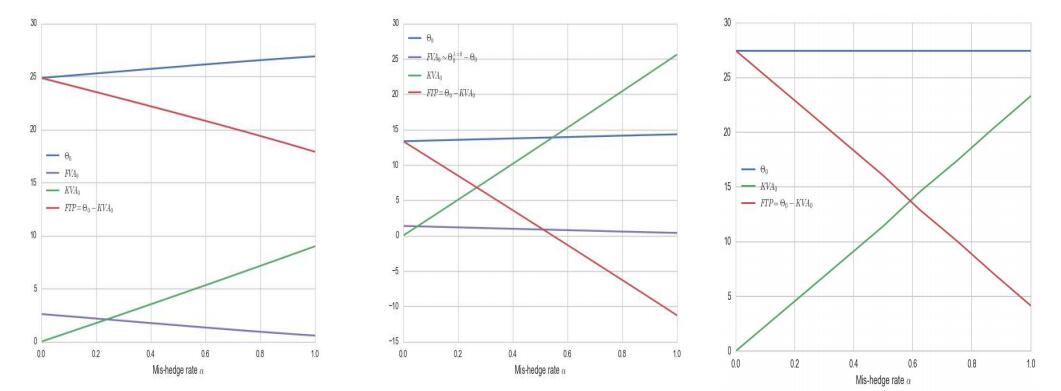
Figure 1: XVAs and FTP as a function of the mis-hedge parameter α. Left: Without
model uncertainty. Middle: With UVM uncertainty (σ uncertainty (σ = 15%, σ = 60%, σ = 30%).Black-Scholes Equations代写
XVA desks, KVA in particular, are the first consulted desks in all major trades today. Our results in a toy model where all the quantities of interest can be computed exactly (modulo the numerical error on the PDE solutions) emphasize that, accounting for model risk, the relative importance of the KVA should become even larger. Moreover one can easily imagine how to transpose these results to the setup of Albanese et al.
(2016) where+each option payoff (STi − Ki) is replaced by the CVA exposure of the bank to the defaultat time of its counterparty i, at the (random) time Ti, with corresponding position of thebank ωiSTi and margins received by the bank ωiKi. However in this case a relevant risk measure really needs to be computed at a one-year horizon (as opposed to instantaneous in(6)), in order to leave time to credit events to develop. This points out to developments of a slightly different nature, which would be interesting to develop.
References Black-Scholes Equations代写
Albanese, C., S. Caenazzo, and S. Cr´epey (2016). Capital valuation adjustment and fund- ing valuation adjustment. arXiv:1603.03012 and ssrn.2745909 (short version “Capital and funding” published in Risk Magazine May 2016, 71-76).
Avellaneda, M., A. Levy, and A. Paras (1995). Pricing and hedging derivative securities in markets with uncertain volatilities. Applied Mathematical Finance 2 (2), 73–88.
Biagini, S., B. Bouchard, C. Kardaras, and M. Nutz (2015). Robust fundamen- tal theorem for continuous processes. Mathematical Finance. Forthcoming (DOI: 10.1111/mafi.12110).
Kruse, T. and A. Popier (2016). BSDEs with monotone generator driven by Brownian and Poisson noises in a general filtration. Stochastics: An International Journal of Probability and Stochastic Processes 88 (4), 491–539.
Peng, S. and Z. Yang (2009). Anticipated backward stochastic differential equations. The Annals of Probability 37 (3), 877–902.
Soner, H., N. Touzi, and J. Zhang (2012). Wellposedness of second order BSDEs. Prob.
Th. and Related Fields 153 (2), 149–190.
Tan, X. and N. Touzi (2013). Optimal transportation under controlled stochastic dynam- ics. The Annals of Probability 41 (5), 3201–3240.
其他代写:考试助攻 计算机代写 java代写 algorithm代写 代写CS assembly代写 function代写paper代写 金融经济统计代写 web代写 数学代写 essay代写 编程代写 report代写 algorithm代写 数学代写 finance代写
