
Financial Modelling 2018-19 Project
Portfolio Optimization
Financial Modelling代写 In our project, we aim to perform a portfolio optimization analysis based on a portfolio of thirty UK stocks and solve seven tasks.

Group members:
Introduction Financial Modelling代写
In our project, we aim to perform a portfolio optimization analysis based on a portfolio of thirty UK stocks and solve seven tasks. In the provided dataset, we have 10 years (Dec. 2007 – Dec. 2017) of monthly price and market capitalization data for each of the stocks as well as prices for the FTSE100 market index and proxies for the risk-free rates over various sub-periods of the sample.
In this report, we offer the clear detailed working process and explanation for efficient frontier generation, portfolio optimization, and out-of-sample risk-adjusted performance analysis. We mainly incorporate Excel Solver and several Excel functions to achieve our results. These tools are extremely effective and next we will present our solution on the seven tasks
Task 1
(1)As required, firstly we calculate return, then we generate variance-covariance matrix for the 30 stocks as shown in table 1.1 (a snapshot of 30*30matrix).
- Our Workings andfindings
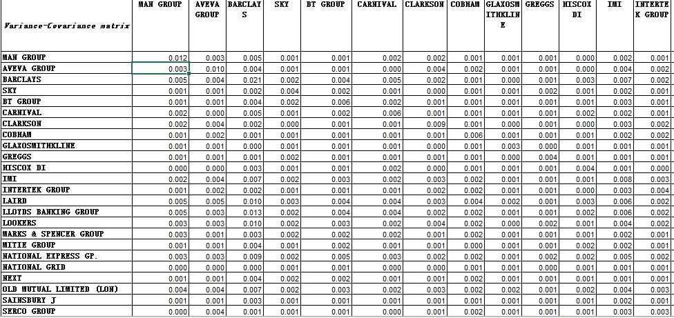
Table 1.1
(2)Then we set up initial weight for each stock as 1/30, and we calculate portfolio statistics using both portfolio return series and Variance-covariance matrix as shown in table2.
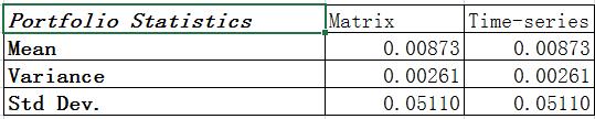
Table 1.2
(3)Use Solver to search for the minimum variance portfolio. The calculated weights are shown in table3.
| MAN GROUP | 0.06691 |
| AVEVA GROUP | 0.05715 |
| BARCLAYS | 0.07092 |
| SKY | -0.00598 |
| BT GROUP | 0.07878 |
| CARNIVAL | 0.07491 |
| CLARKSON | 0.06324 |
| COBHAM | 0.00904 |
| GLAXOSMITHKLINE | 0.09425 |
| GREGGS | 0.08846 |
| HISCOX DI | 0.11716 |
| IMI Financial Modelling代写 | -0.04639 |
| INTERTEK GROUP | 0.17510 |
| LAIRD | -0.01576 |
| LLOYDS BANKING GROUP | 0.01236 |
| LOOKERS | 0.00323 |
| MARKS & SPENCER GROUP | -0.01161 |
| MITIE GROUP | 0.02741 |
| NATIONAL EXPRESS GP. | -0.04591 |
| NATIONAL GRID | 0.30425 |
| NEXT | 0.01086 |
| OLD MUTUAL LIMITED (LON) | -0.16427 |
| SAINSBURY J | 0.12681 |
| SERCO GROUP | 0.00261 |
| SHIRE | 0.06211 |
| SIG | -0.05674 |
| UNILEVER (UK) | -0.00701 |
| UNITE GROUP | -0.04049 |
| VESUVIUS | -0.03559 |
| WILLIAM HILL | -0.01579 |
Table 1.3
(4)Set up the target standard deviation and use Solver to maximize and minimize return for portfolios, then plot return against variance and get the efficient frontier graph as shown in graph 1.1.
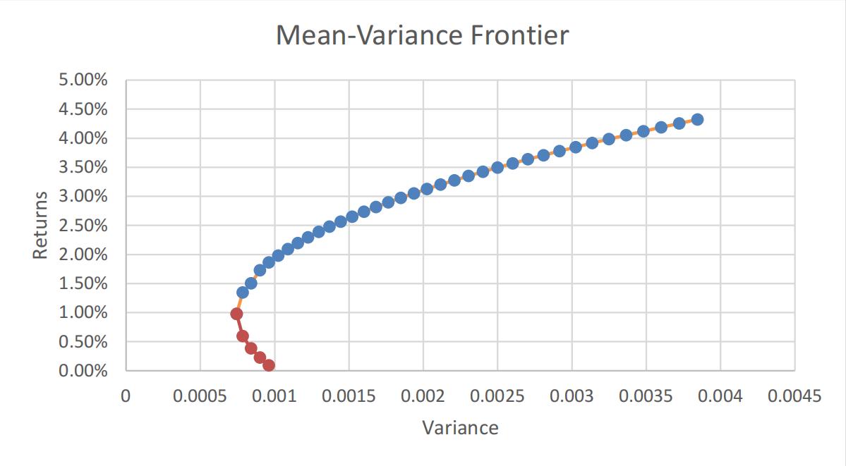
Graph 1.1
(5)Calculate 30 stocks return and variance and then plot them in the same efficient frontier graph as shown in graph 1.2
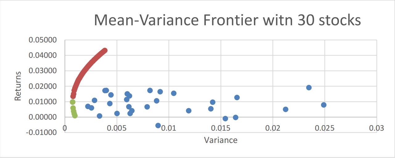
Graph 1.2
As we can see, the mean-variance frontier generates a much better risk-adjusted return and this shows that firm specific risks of these 30 stocks tend to offset each other and expected returns are not sacrificed. Based on what we have learnt, the unsystematic risks fade away when we add more and more risky asset into our portfolio: the benefits of diversification.

Task 2
- Our workings and findings
(1)Paste price data and risk-free rate data into a new worksheet and calculate returns for 30 stocks. Then we set up initial weight for each stock as 1/30 and create a portfolio column with MMULT function
(2)Create Variance-covariance matrix using MMULT function on the returnseries
(3)Calculate portfolio statistics using both portfolio return seriesand Variance-covariance matrix to double check the result as shown in table 2.1.

Table 2.1
(4)Use Solver to search for the maximum Sharpe ratio portfolio and the weights for each stock are shown in table 2.2 But we do not believe that the composition of the market portfolio that we have found is a desirable or practical one as an investment. The reasons are we need to short 15 stocks, and the short-selling will be very costly since we need to put the money in margin account and we may have margin call. Further, we need to monitor and manage 30 stocks, and this will be very time-consuming and hard.
| The Market Portfolio (M) | |
| MAN GROUP | 0.1313832 |
| AVEVA GROUP | 0.2085357 |
| BARCLAYS | -0.1108155 |
| SKY | -0.1383923 |
| BT GROUP | 0.1557715 |
| CARNIVAL | 0.2185837 |
| CLARKSON | 0.0269352 |
| COBHAM | -0.2845411 |
| GLAXOSMITHKLINE | -0.0331599 |
| GREGGS | 0.1826932 |
| HISCOX DI | 0.6554072 |
| IMI | 0.2024278 |
| INTERTEK GROUP | 0.6231719 |
| LAIRD | -0.0656085 |
| LLOYDS BANKING GROUP | -0.1508879 |
| LOOKERS | 0.1295702 |
| MARKS & SPENCER GROUP | -0.3237494 |
| MITIE GROUP | -0.2175324 |
| NATIONAL EXPRESS GP. | -0.0585352 |
| NATIONAL GRID | 0.1941891 |
| NEXT Financial Modelling代写 | 0.4516032 |
| OLD MUTUAL LIMITED (LON) | -0.1970358 |
| SAINSBURY J | -0.1675147 |
| SERCO GROUP | -0.2786533 |
| SHIRE | 0.1528195 |
| SIG | -0.1094252 |
| UNILEVER (UK) | -0.2214737 |
| UNITE GROUP | 0.0392485 |
| VESUVIUS | -0.0208471 |
| WILLIAM HILL | 0.0058319 |
Table 2.2
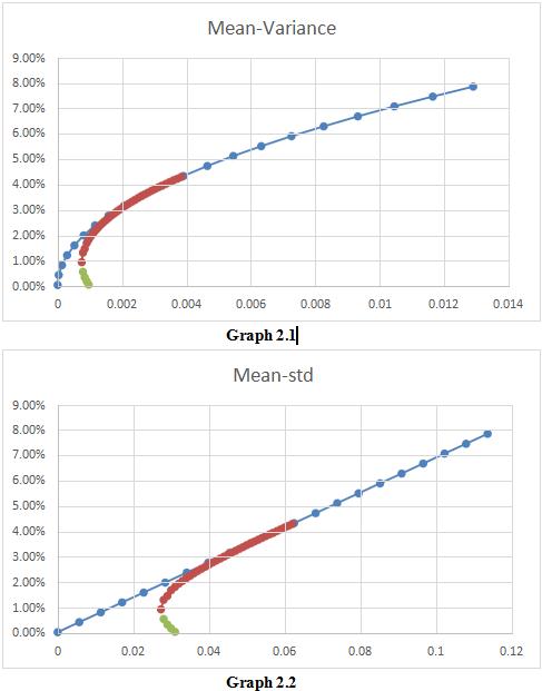
(5)Set up the different weight for risk-free asset and calculate weight for risky asset, and portfolio return and variance. Then we plot investor portfolio return against variance and standard deviation, and add them on the efficient frontier graph as shown in graph 2.1 and 2.2. As we can see, based on two fund separation theorem, the introduction of risk-free asset changes the optimal portfolio holdings for investors from red line to blue line (capital marketline).
Task 3
⚫ Our workings and findings
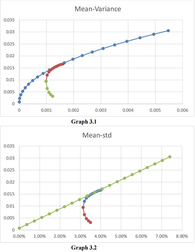
(1)We repeat steps from task 1 to task 2, but restricting short selling. The composition of market portfolio is shown in table 3.1. As we can see this portfolio only has long position so we do not need to short any stocks. Further, we only need to invest in 8 stocks, so our management and transaction costs will be lower than previous portfolio, which has 30 positions to invest and manage. In conclusion, the portfolio restricting short selling is the more desirable or practical portfolio as an investment.
| The Market Portfolio (M) | |
| MAN GROUP | 0.0000000 |
| AVEVA GROUP | 0.0149952 |
| BARCLAYS | 0.0000000 |
| SKY | 0.0000000 |
| BT GROUP | 0.0000000 |
| CARNIVAL | 0.0000000 |
| CLARKSON | 0.0716133 |
| COBHAM | 0.0000000 |
| GLAXOSMITHKLINE | 0.0000000 |
| GREGGS | 0.1461971 |
| HISCOX DI | 0.2997616 |
| IMI | 0.0000000 |
| INTERTEK GROUP | 0.2643230 |
| LAIRD | 0.0000000 |
| LLOYDS BANKING GROUP | 0.0000000 |
| LOOKERS | 0.0000000 |
| MARKS & SPENCER GROUP | 0.0000000 |
| MITIE GROUP | 0.0000000 |
| NATIONAL EXPRESS GP. | 0.0000000 |
| NATIONAL GRID | 0.0705641 |
| NEXT | 0.0879743 |
| OLD MUTUAL LIMITED (LON) | 0.0000000 |
| SAINSBURY J | 0.0000000 |
| SERCO GROUP | 0.0000000 |
| SHIRE | 0.0445714 |
| SIG | 0.0000000 |
| UNILEVER (UK) | 0.0000000 |
| UNITE GROUP | 0.0000000 |
| VESUVIUS | 0.0000000 |
| WILLIAM HILL | 0.0000000 |
Table 3.1
(2)We also plot the capital market line and efficient frontier as shown ingraph 3.1 and 3.2.
Task 4 Financial Modelling代写
⚫ Our workings and findings
(1)We Divide the sample in first half (Jan. 2008-Dec. 2012, “in-sample period”) and second half Jan. 2013-Dec. 2017, “out-of-sampleperiod”).
(2)Then we construct equally-weighted portfolios andmarket capitalization-weighted portfolios of the 30 stocks for both sub-sample periods.
(3)We compare the risk-adjusted performance of these four portfolios using Sharpe ratio as shown in table1 4.1
| Sharpe Ratio Difference | Jan. 2008-Dec. 2012 | Jan. 2013-Dec. 2017 | Market Weighted Portfolio |
| Jan. 2008-Dec. 2012 | 0.040 | -0.144 | |
| Jan. 2013-Dec. 2017 | 0.251 | 0.067 | |
| Equal Weighted Portfolio |
Table 4.1
As we can see, equal weighted portfolio outperforms market capitalization weighted portfolios in both in-sample and out-of-sample period since its Sharpe ratios are higher than later. Further, the Sharpe ratio difference even increases in out-of-sample period and this shows that equal-weighted portfolio is more stable.
Task 5
⚫ Our workings and findings
(1)We repeat steps in task 3 but this time we re-estimate the market portfolio and the minimum variance portfolio using the first half of the data only(Jan.2008-Dec.2012). The weights of both portfolios are shown below in table 5.1 and 5.2.
| Minimum Variance Portfolio Weights | |
| MAN GROUP | 0.0276759 |
| AVEVA GROUP | 0.0000000 |
| BARCLAYS | 0.0000000 |
| SKY Financial Modelling代写 | 0.0000000 |
| BT GROUP | 0.0000000 |
| CARNIVAL | 0.0000000 |
| CLARKSON | 0.0000000 |
| COBHAM | 0.0000000 |
| GLAXOSMITHKLINE | 0.1599254 |
| GREGGS | 0.1618785 |
| HISCOX DI | 0.0141122 |
| IMI | 0.0000000 |
| INTERTEK GROUP | 0.0772122 |
| LAIRD | 0.0000000 |
| LLOYDS BANKING GROUP | 0.0000000 |
| LOOKERS | 0.0000000 |
| MARKS & SPENCER GROUP | 0.0000000 |
| MITIE GROUP | 0.1304072 |
| NATIONAL EXPRESS GP. |
0.0000000 |
| NATIONAL GRID | 0.3232745 |
| NEXT | 0.0000000 |
| OLD MUTUAL LIMITED (LON) | 0.0000000 |
| SAINSBURY J | 0.1055140 |
| SERCO GROUP | 0.0000000 |
| SHIRE | 0.0000000 |
| SIG | 0.0000000 |
| UNILEVER (UK) | 0.0000000 |
| UNITE GROUP | 0.0000000 |
| VESUVIUS | 0.0000000 |
| WILLIAM HILL | 0.0000000 |
Table 5.1
| Market Portfolio Weights | |
| MAN GROUP | 0.0000000 |
| AVEVA GROUP | 0.1230718 |
| BARCLAYS | 0.0000000 |
| SKY | 0.0000000 |
| BT GROUP | 0.0000000 |
| CARNIVAL | 0.0000000 |
| CLARKSON Financial Modelling代写 | 0.0000000 |
| COBHAM | 0.0000000 |
| GLAXOSMITHKLINE | 0.0000000 |
| GREGGS | 0.0000000 |
| HISCOX DI | 0.2007059 |
| IMI | 0.0000000 |
| INTERTEK GROUP | 0.4471119 |
| LAIRD | 0.0000000 |
| LLOYDS BANKING GROUP | 0.0000000 |
| LOOKERS | 0.0000000 |
| MARKS & SPENCER GROUP | 0.0000000 |
| MITIE GROUP | 0.0000000 |
| NATIONAL EXPRESS GP. |
0.0000000 |
| NATIONAL GRID | 0.0000000 |
| NEXT | 0.2291104 |
| OLD MUTUAL LIMITED (LON) | 0.0000000 |
| SAINSBURY J | 0.0000000 |
| SERCO GROUP | 0.0000000 |
| SHIRE | 0.0000000 |
| SIG | 0.0000000 |
| UNILEVER (UK) | 0.0000000 |
| UNITE GROUP | 0.0000000 |
| VESUVIUS | 0.0000000 |
| WILLIAM HILL | 0.0000000 |
Table 5.2
(2)We then Use the weights of the market portfolio and the minimum variance portfolio from the first half of the data and apply those to the second half of the data (Jan. 2013-Dec.2017)
(3)We compare the risk-adjusted performance of the four portfolios using the Sharpe ratio as shown in table 5.3
| Sharpe Ratio Analysis for | two periods | ||||
| Minimum Variance Portfolio | Mean | Std | Risk Free rate | Risk Premium | Sharpe Ratio |
| Jan. 2008-Dec. 2012 | 0.56% | 0.033152915 | 0.11% | 0.45% | 0.134792068 |
| Jan. 2013-Dec. 2017 | 0.96% | 0.03115284 | 0.03% | 0.93% | 0.300043555 |
| Market Portfolio | Mean | Std | Risk Free rate | Risk Premium | Sharpe Ratio |
| Jan. 2008-Dec. 2012 | 0.020 | 0.048005271 | 0.11% | 1.90% | 0.39651647 |
| Jan. 2013-Dec. 2017 | 0.012920542 | 0.041058505 | 0.03% | 1.26% | 0.307379471 |
| Sharpe ratio difference | Jan. 2008-Dec. 2012 | Jan. 2013-Dec. 2017 | << Minimum Variance Portfolio |
| Jan. 2008-Dec. 2012 | 0.261724401 | 0.096472915 | |
| Jan. 2013-Dec. 2017 | 0.172587402 | 0.007335916 | |
| Market Portfolio ^^ |
Table 5.3
As we can see, market portfolio outperforms minimum variance portfolio a lot in in-sample period, but in out-of-sample period, it only beats later a little. This shows that the maximum Sharpe ratio strategy is not stable and we need to be careful when using this strategy in long-term investment.
Task 6 Financial Modelling代写
⚫ Our workings and findings
(1) We rank the portfolio performance based on Sharpe ratio as shown in table 6.1 and present the detailed Sharpe ratio table in table 6.2
| Rankings | |
| Sharpe ratio for in-sample | Sharpe ratio for out-sample |
| Market Portfolio | Market Portfolio |
| Minimum Variance Portfolio | Equal Weighted Portfolio |
| Equal Weighted Portfolio | Minimum Variance Portfolio |
| Market capitalisation-Weighted Portfolio | Market capitalisation-Weighted Portfolio |
Table 6.1
| Sharpe Ratio Analysis for two periods | |
| Equal Weighted Portfolio | Sha rp e R a tio |
| Jan. 2008-Dec. 2012 | 0.09570 |
| Jan. 2013-Dec. 2017 | 0.30669 |
| Market capitalisation-Weighted Portfolio | Sha rp e R a tio |
| Jan. 2008-Dec. 2012 | 0.05597 |
| Jan. 2013-Dec. 2017 | 0.23925 |
| Minimum Variance Portfolio | Sha rp e R a tio |
| Jan. 2008-Dec. 2012 | 0.13479 |
| Jan. 2013-Dec. 2017 | 0.30004 |
| Market Portfolio | Sha rp e R a tio |
| Jan. 2008-Dec. 2012 | 0.39652 |
| Jan. 2013-Dec. 2017 | 0.30738 |
Table 6.2
As we can see, the market portfolio outperforms all other strategy in both the in-sample and out-sample period,
but it actually performs worse than pervious period (with global financial crisis), so this is a surprise to us and may show that the estimated weight for market portfolio only suits for the similar market conditions. If the market conditions change, the market portfolio can not perform as good as it was. The Sharpe ratio difference among four strategies also shrink in out-of-sample period. As Victor DeMiguel says in his paper, Optimal Versus Naive Diversification: How Inefficient is the 1/N Portfolio Strategy?, the gain from optimal diversification is more than offset by estimation error with time. We are also amazed by the performance of naive equal-weighted portfolio as we will discuss next. Financial Modelling代写
Further, As ROGER C LARKE et al. presented in their paper, Risk Parity, Maximum Diversification, and Minimum Variance: An Analytic Perspective, from 1986 to 2012, equal-weighted portfolio outperforms market capitalization-Weighted Portfolio but underperforms Minimum Variance Portfolio in risk-adjusted basis. But in our results, we can see that equal-weighted portfolio performs better than minimum variance portfolio in resurgence period but worse than minimum variance portfolio in recession. We think this makes sense since the minimum variance portfolio limits the big downside risk but also restrains the upside returns. This is why our results are not what we have expected
Conclusion
After the long-term working on financial modeling, and analysis on different portfolio strategy (such as minimum Variance, maximum Sharpe ratio, equally-weighted and market capitalization-weighted), we have learnt how to merge theory with practice and conduct further research in empirical literature to solve our questions. We sincerely appreciate this project and will continuously reflect on our work throughout our future life.
References Financial Modelling代写
1.Clarke, Roger G and de Silva, Harindra and Thorley, Steven, RiskParity,Maximum Diversification, and Minimum Variance: An Analytic Perspective (June 1, 2012). Journal of Portfolio Management, Vol. 39, No. 3, pp. 39-53 (Spring 2013).
Available at SSRN: https://ssrn.com/abstract=1977577 or http://dx.doi.org/10.2139/ssrn.1977577
2.DeMiguel, Victor and Garlappi, Lorenzo and Uppal, Raman, Optimal Versus Naive Diversification: How Inefficient is the 1/N Portfolio Strategy? (May 2009). The Review of Financial Studies, Vol. 22, Issue 5, pp. 1915-1953, 2009. Available at SSRN: https://ssrn.com/abstract=1376199 orhttp://dx.doi.org/hhm075